Model types for the inversion of TEM/FEM data in Aarhus Workbench

Most inversions are done with smooth models only, but often the resolution is good enough to sense more abrupt changes in the geology than the smooth model can allow for. This can make the use of subsequent inversions with layered models interesting for complementary insights about the subsurface. We will look at layered models, block models and briefly sharp models, as well as an option to create individual layered models from existing smooth models.

Overview

[00:00:02.320]
<v ->Hello, thanks for joining this presentation.</v>

[00:00:05.650]
My name is Bjarke Roth and I’m a geophysicist

[00:00:07.910]
with Aarhus GeoSoftware.

[00:00:10.191]
Today we are going to look at model types

[00:00:12.000]
as we use them for inversions in Aarhus Workbench.

[00:00:15.970]
Let’s say that we have measured some data,

[00:00:18.040]
it could be did TDEM soundings, like this one,

[00:00:21.090]
from an airborne time-domain EM system,

[00:00:23.350]
or it could be a frequency domain EM systems.

[00:00:28.060]
And we have spent some time to remove couplings

[00:00:30.740]
and noise from the data

[00:00:32.368]
so that it not only reflects the geology.

[00:00:35.900]
Before we can pass it on,

[00:00:37.030]
we need to turn it into a physical model of the subsurface

[00:00:40.290]
that a geologist then can use

[00:00:41.530]
to create the more elaborate models that they work on.

[00:00:45.450]
Unfortunately, there is no straightforward way to do that.

[00:00:48.440]
And in fact,

[00:00:49.273]
it turns out to be much easier to go the other way.

[00:00:52.570]
We know the physics and with an accurate system description

[00:00:57.320]
it’s possible to calculate the forward response

[00:00:59.040]
that one would measure for a given model.

[00:01:01.330]
So, what we can do is to compare this forward response

[00:01:04.450]
with the measured data.

[00:01:07.000]
We do this comparison with an objective function,

[00:01:09.360]
an example of that is this data residual.

[00:01:12.260]
Here we compared the observed data and the forward data

[00:01:14.870]
and we normalize it with the data uncertainty.

[00:01:17.220]
Really the C here is the diagonal entries

[00:01:19.610]
in the covarience matrix,

[00:01:20.760]
but it contains the data uncertainty squared.

[00:01:23.590]
A value of one

[00:01:24.423]
means that the data have fitted within the noise.

[00:01:26.680]
Anything below one is, in that sense, equally correct.

[00:01:30.060]
A value equal to two

[00:01:31.100]
means that data have fitted

[00:01:32.527]
with an interval of two times to noise and so on.

[00:01:35.568]
By minimizing this function,

[00:01:36.510]
we will find the version of our model

[00:01:38.740]
that comes closest to giving us the data we have observed.

[00:01:43.480]
The simplest 1D model we can have is a half space model,

[00:01:46.950]
that is a model with only one resistivity parameter

[00:01:49.210]
to describe the subsurface.

[00:01:51.510]
So let’s have a quick and somewhat simplified look

[00:01:53.770]
at how the inversion process works for the situation.

[00:01:57.698]
If we could calculate the data residual

[00:02:00.040]
for all allowed residual values it might look like this,

[00:02:03.550]
but inversion cannot see this curve.

[00:02:06.434]
Instead it will, for each iteration,

[00:02:08.700]
calculate the data residual

[00:02:11.620]
and then the derivative for the model parameter.

[00:02:14.910]
And then it can adjust the resistivity model parameter

[00:02:17.550]
based on that derivative taking a jump into subspace.

[00:02:21.580]
This repeats and repeats

[00:02:25.970]
until it cannot improve the result anymore.

[00:02:30.160]
And hopefully it ends up in the global minimum

[00:02:34.660]
rather than a local minimum.

[00:02:38.470]
This approach is called Levenberg-Marquardt algorithm

[00:02:41.120]
or damped least-square.

[00:02:42.820]
I have included a few references

[00:02:44.300]
for anyone who’s interested in those.

[00:02:47.040]
It doesn’t always find a global minimum,

[00:02:48.780]
but it is quite robust for where well behaved functions

[00:02:51.240]
and reasonable starting parameters.

[00:02:53.480]
And in most cases,

[00:02:54.313]
the functions we work with will be fairly well behaved.

[00:02:57.410]
You can, however, in some cases, end up in situations

[00:03:00.710]
where you need to improve your starting model

[00:03:02.670]
to not end up in a local minimum.

[00:03:05.839]
We, of course, usually want a little more detail

[00:03:08.450]
in our 1D models than just the one resistivity parameter.

[00:03:12.180]
Conceptually, the simplest model is the layered model

[00:03:14.410]
where we have a few layers,

[00:03:16.050]
each layer having a resistivity and a thickness.

[00:03:19.000]
Unfortunately, it is not easiest model type to work with.

[00:03:22.480]
The layers you end up with

[00:03:23.520]
will not always correspond directly

[00:03:25.240]
to the overall geological layers,

[00:03:27.250]
so it takes practice and understanding of subsurface

[00:03:29.730]
to get it right.

[00:03:31.130]
But we will talk more about why that is so in a bit.

[00:03:34.820]
Instead,

[00:03:35.653]
we will turn to the smooth model as our starting point.

[00:03:39.120]
Here we have more layers, 20 to 40 depending on data type,

[00:03:43.040]
but only the resistivities is estimated.

[00:03:45.470]
The thicknesses are kept fixed

[00:03:46.770]
with increasing size with depth.

[00:03:48.720]
And the resistivities also vertical constrained

[00:03:50.670]
to ensure continuity between the layers,

[00:03:53.000]
hence to name smooth.

[00:03:55.760]
Let us unpack this a little.

[00:03:57.453]
There’s a big advantage to this approach.

[00:04:00.230]
The starting conditions are much less important

[00:04:02.940]
than for the layered models.

[00:04:05.850]
We of course have the starting resistivities

[00:04:07.440]
of all these layers,

[00:04:08.950]
but we almost always use a uniform starting model

[00:04:11.990]
to not introduce structure in the model with resistivities.

[00:04:14.630]
And as long as we don’t get too far away

[00:04:16.750]
from where we need to go with the resistivities,

[00:04:19.050]
this will just translate

[00:04:20.400]
into slightly longer inversion times

[00:04:22.980]
as the inversion needs to take a few extra iterations

[00:04:25.770]
to change resistivities and we do have some options

[00:04:29.930]
for improving that starting model,

[00:04:32.227]
those starting resistivities.

[00:04:34.580]
More importantly, because the layers are fixed,

[00:04:36.970]
the layer setup is not as important for the final model,

[00:04:40.870]
the final smooth model, as it is for a layered model.

[00:04:46.663]
All we need to decide for the setup is

[00:04:48.590]
the first layer boundary, the last layer boundary,

[00:04:50.590]
the number of layers, and the vertical constraints,

[00:04:53.430]
all of which we can do relatively objectively

[00:04:55.610]
based on the used instrument and data type.

[00:04:58.960]
The expected near surface resolution

[00:05:00.468]
give us the first layer boundary,

[00:05:02.950]
if we make this too thin,

[00:05:04.300]
it will just be determined by the starting value

[00:05:06.720]
and the constraints.

[00:05:08.680]
The deepest expected depth of penetration

[00:05:11.100]
give us the last layer boundary,

[00:05:13.170]
again, if we make this too deep,

[00:05:14.900]
it will just be determined by the starting value

[00:05:17.010]
and the constraints.

[00:05:18.140]
And we can sort that away

[00:05:19.640]
without depth of investigation measure later on.

[00:05:23.090]
But if you don’t make it deep enough,

[00:05:25.813]
we will not be able to fit the late term data.

[00:05:30.050]
The expected resolution give us an idea about the number of layers

[00:05:33.500]
to use, this also ties into the vertical constraints.

[00:05:37.660]
They are there to stabilize inversion

[00:05:39.940]
and reduce overshoot/undershoot effects

[00:05:41.850]
we might otherwise see with poorly resolved layers.

[00:05:44.850]
This can, however, again, be set relative objectively

[00:05:47.550]
based on the expected geological variation.

[00:05:50.486]
Then it’s simply a matter of entering the numbers

[00:05:52.680]
into a model discretization calculator

[00:05:55.020]
and let it distribute the layers

[00:05:56.810]
so that the increase thickness discretization

[00:06:00.940]
down through the model.

[00:06:04.770]
I talked about constraints,

[00:06:06.304]
but not really explained what they are.

[00:06:09.070]
All our constraints work like factors.

[00:06:10.930]
A value of two means that to resistivity of the layer above

[00:06:13.810]
or below are allowed one sigma interval on its resistivity

[00:06:17.340]
going from the layer of resistivity divided by two

[00:06:19.840]
to the layer of resistivity multiplied by two.

[00:06:22.070]
So it’s not a hard limit.

[00:06:23.280]
It can in principle change quicker than that,

[00:06:25.713]
but it’ll be more costly for inversion to do so.

[00:06:30.890]
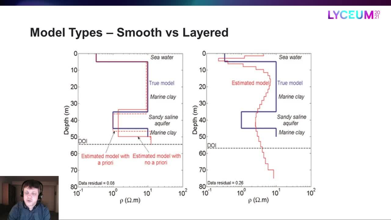
Let’s have a look at an example.

[00:06:32.980]
The blue line is the true model

[00:06:34.470]
while the red line is estimated smooth model.

[00:06:37.340]
The DOI is the depth of investigation

[00:06:39.770]
that I briefly mentioned earlier,

[00:06:41.390]
which is the depth to which we can trust the results

[00:06:44.130]
to mainly depend on the data

[00:06:45.920]
rather than the starting values and constraints.

[00:06:49.300]
So the smooth model type reproduced the overall structure,

[00:06:53.149]
but we’re not exactly getting the correct layer transitions

[00:06:56.160]
and layer resistivities here.

[00:06:59.730]
Now let us compare that with estimate layered model.

[00:07:03.240]
Here we actually have two layered models,

[00:07:05.800]
one without a priori

[00:07:07.010]
and one where they resistivity of the third layer

[00:07:08.840]
was used to help the inversion in the right direction.

[00:07:13.290]
So clearly the layered model

[00:07:15.230]
can get much better layer transitions and resistivities,

[00:07:18.360]
particularly if we help it along.

[00:07:22.640]
If we, however, start the inversion with layer thickness

[00:07:25.360]
that are too far off,

[00:07:26.640]
it can end up placing the layer transitions differently

[00:07:29.340]
and wasting layers where we don’t really need them.

[00:07:32.220]
This situation can be improved

[00:07:33.670]
with the knowledge of the overall structure

[00:07:35.470]
that we can get from the smooth model,

[00:07:37.200]
but it can take a few attempts to get it right.

[00:07:40.717]
One can either use the first

[00:07:42.960]
and last layer boundary approach

[00:07:44.829]
or edit the layers individually,

[00:07:47.060]
but it tends to be more trial and error

[00:07:49.300]
than the smooth model set up,

[00:07:51.440]
perhaps because the layered model,

[00:07:52.650]
more so than a smooth model,

[00:07:53.940]
reflects the nativity of your data.

[00:07:56.190]
So make sure to focus your setup efforts on the top part

[00:08:00.300]
of the model where most of nativity of your data

[00:08:02.340]
will be reflected.

[00:08:05.150]
So looking at these two model types,

[00:08:06.940]
we are left with “all models are wrong, some are useful”.

[00:08:10.600]
Neither of these models hold all the answers,

[00:08:12.750]
but both models give useful

[00:08:14.810]
and somewhat complimentary insights about the subsurface.

[00:08:20.317]
Now let us broaden the approach a little

[00:08:22.540]
before we look at the last two model types.

[00:08:25.250]
We often invert a lot of models at the same time

[00:08:27.550]
so we of course need to talk about

[00:08:29.400]
how lateral constraints enter into this.

[00:08:31.229]
We expect a certain continuity in the geology.

[00:08:34.638]
It will depend on the specific geology of course,

[00:08:37.610]
but we expect models next to each other

[00:08:39.670]
to have some similarities.

[00:08:41.960]
We can either have constraints along the flight line,

[00:08:45.480]
this is called lateral constrained inversion or LCI.

[00:08:48.894]
Or we can have constraints both along the flight lines

[00:08:51.030]
and between the flight lines,

[00:08:52.280]
this is called a spatially constrained inversion or SCI.

[00:08:55.680]
Both of these are still 1D inversions,

[00:08:58.040]
the forward calculation here is still done in 1D.

[00:09:01.710]
But the models become quasi 2D for LCI and quasi 3D for SCI.

[00:09:07.920]
In practice,

[00:09:08.760]
the SCI constraints will look something like this.

[00:09:12.013]
The red points are the model positions

[00:09:13.860]
and the black lines are the constraints.

[00:09:16.380]
The constraints are determined with an algorithm,

[00:09:18.070]
it ensures that we get a structure like this,

[00:09:20.950]
where we always have constraints along the flight lines

[00:09:23.310]
as well as to nearby flight lines.

[00:09:26.300]
One important detail here is

[00:09:27.770]
that unlike with the vertical constraints

[00:09:29.910]
distance clearly needs to be considered here.

[00:09:32.490]
We don’t want the constraints to be equally strong

[00:09:34.320]
between all model positions.

[00:09:36.640]
So we set a reference distance for our inversion.

[00:09:39.950]
Any constraints between models

[00:09:41.760]
that stay within that distance, use the fact as given,

[00:09:46.270]
while the models further apart

[00:09:47.740]
will have that constraint scaled to become weaker.

[00:09:51.290]
If we set this reference distance

[00:09:52.710]
equal to the average sounding distance between our models

[00:09:55.400]
along the flight line,

[00:09:56.750]
the lateral constraint can be set

[00:09:58.650]
based on the expected amount of geological variation

[00:10:01.490]
in the area, rather than being some arbitrary factor.

[00:10:05.100]
The scaling will then take care of the rest of us.

[00:10:08.350]
For some data type

[00:10:09.210]
this reference distance is calculated automatically,

[00:10:11.770]
but, in other cases, it is part of the model setup.

[00:10:15.580]
Something like the altitude is also constrained,

[00:10:18.440]
but those constraints are kept separate

[00:10:20.090]
and only constraint along the flight lines.

[00:10:25.480]
Now we’re able to put all the pieces together.

[00:10:27.920]
When we talked about inversion earlier,

[00:10:29.830]
we used a simple objective function

[00:10:31.570]
that only looked at data residual.

[00:10:33.930]
The full objective function

[00:10:35.200]
most of course also take the constraints

[00:10:37.520]
and the a priori into account.

[00:10:39.850]
Just as the data residual compares observed and forward data

[00:10:45.229]
normalized with the data uncertainty,

[00:10:47.390]
the constraint parts

[00:10:48.990]
compares the constraint model parameters

[00:10:54.656]
normalized with the factor

[00:10:56.095]
set for the strength of those constraints.

[00:10:59.296]
And a priori part compares model parameters

[00:11:01.551]
with a priori for those model parameters

[00:11:03.903]
normalized with the factors

[00:11:05.610]
set for the strength of those a priori.

[00:11:09.310]
The constraint part is the most interesting here

[00:11:11.430]
as it highlights a few differences between the layered

[00:11:14.370]
and smooth models.

[00:11:16.190]
We have vertical constraints on resistivities

[00:11:18.000]
but only for smooth models.

[00:11:19.430]
We have lateral constraints on resistivities,

[00:11:21.389]
this is used by both layered and smooth models.

[00:11:24.320]
And we have lateral constraint on the layer thickness

[00:11:26.120]
of all layer depths, but only for layered models.

[00:11:30.240]
Both the thickness

[00:11:31.073]
and depth approach for the layered model works,

[00:11:33.090]
but there are, of course, some differences in setup

[00:11:35.930]
when we used factors on depth of all the layers above

[00:11:39.130]
rather than just the thickness of the individual layers

[00:11:43.130]
that is detailed however.

[00:11:44.990]
The constraint part is also interesting

[00:11:47.030]
because it is the basis for the two last model types.

[00:11:52.120]
The idea with both of them is to have a model

[00:11:54.880]
that you set up similar to how you set up a smooth model,

[00:11:58.306]
without needing to know much

[00:12:00.150]
about where the layer transitions should be,

[00:12:02.710]
but where the end result

[00:12:03.950]
takes on more of the characteristics of the layout result

[00:12:06.730]
with the more distinct layers.

[00:12:10.790]
The simplest approach is called a blocky model

[00:12:13.040]
and it is really surprising simple.

[00:12:16.030]
Rather than using the squared difference

[00:12:20.067]
it uses the absolute difference for the constraints part.

[00:12:24.720]
I have plotted the penalty cost of the sum terms here.

[00:12:27.257]
So what we are looking at is the penalty

[00:12:30.217]
given the absolute difference of the model parameters

[00:12:33.730]
normalized with the facts that we have set

[00:12:35.930]
for the constraints.

[00:12:37.640]
Clearly there two regions here.

[00:12:39.370]
When we are above one

[00:12:42.710]
the blocky model has a much lower penalty.

[00:12:47.740]
So it can, in that sense, allow much larger model changes

[00:12:51.260]
then the smooth model.

[00:12:54.920]
When we are below one

[00:12:55.910]
the blocky model has a slightly higher penalty,

[00:12:58.980]
so it can, in that sense,

[00:13:00.330]
not allow as large or small changes as the smooth model.

[00:13:05.090]
And that is exactly what we see.

[00:13:06.780]
Here we have a smooth model, a blocky model,

[00:13:09.607]
and a layered model inversion result

[00:13:12.160]
all of the same sounding.

[00:13:13.577]
The blocky model changes more,

[00:13:17.250]
changes the resistivity more quickly

[00:13:20.120]
and it stays more flat once it has made that change

[00:13:24.500]
than the smooth model.

[00:13:28.270]
It has the exact same setup as the smooth model

[00:13:30.749]
but gives us something that is a little closer

[00:13:33.930]
to the layered model in result.

[00:13:36.890]
In fact, the setup is so close to the smooth model setup

[00:13:39.440]
that we can take a copy of this, a smooth model SCI,

[00:13:43.750]
and just flip one switch to invert it as a blocky model.

[00:13:50.270]
Here, we have them not just for a single model

[00:13:53.380]
but over a line with 3.2 kilometers of SkyTEM data.

[00:13:57.700]
The layered model is struggling a bit

[00:14:00.140]
in a few transitions areas,

[00:14:02.530]
but otherwise the results look quite good

[00:14:04.790]
for all the model types.

[00:14:09.300]
The last approach is called a sharp model.

[00:14:12.690]
As you can see, for this it gets a little more complicated,

[00:14:16.810]
so I’ll not try to cover all the details.

[00:14:20.980]
I have again plotted the penalty costs of the sum terms,

[00:14:25.394]
or at least most of it,

[00:14:26.970]
as I’ll likely will be ignoring the beta value here.

[00:14:32.090]
This time the penalty stays closer to the smooth curve

[00:14:39.220]
for small values, but it fans out for larger values.

[00:14:43.630]
So once we get about one or so

[00:14:46.490]
it effectively becomes the number of variations

[00:14:48.810]
rather than the total amount of variation

[00:14:51.090]
that is added to the penalty cost.

[00:14:55.530]
This approach is called minimum gradient support.

[00:14:59.320]
In practice, we get a set of sharpness parameters,

[00:15:03.200]
one with a vertical sharpness

[00:15:04.520]
and one with a lateral sharpness.

[00:15:06.620]
These are related to this beta value I skipped over.

[00:15:09.394]
They influence how many blocks you get.

[00:15:11.808]
While they’re used for vertical and lateral constraints

[00:15:15.260]
affect the amount of variation within the blocks.

[00:15:18.060]
The number of blocks is, however, rather data-driven,

[00:15:20.410]
so it’s more like you set

[00:15:21.808]
how distinct it should make the blocks

[00:15:24.040]
than actually how many blocks.

[00:15:26.177]
Let us see some results.

[00:15:29.220]
Depending on the setup

[00:15:30.320]
the result can go from being very similar to a smooth model

[00:15:34.340]
to something like this,

[00:15:35.599]
where it ends up pretty close to the layered model.

[00:15:39.330]
It can change resistivities very quickly,

[00:15:41.873]
but, it is, of course, still limited by the resolution

[00:15:46.100]
of the fixed layers we have given it.

[00:15:50.580]
It is just like the smooth model in that regard,

[00:15:53.530]
but it certainly can come closer to the layered model

[00:15:55.950]
in result.

[00:15:57.400]
It does take some getting used to.

[00:15:59.050]
The numerical values for the sharpness parameters

[00:16:01.210]
are somewhat different from the constraints,

[00:16:03.540]
but there are suggestions for usable values on the F1 Wiki,

[00:16:06.970]
you can open from Aarhus Workbench.

[00:16:09.670]
Lateral values will make the blocks more distinct.

[00:16:12.657]
The usual vertical and lateral constraints

[00:16:14.840]
end up requiring smaller numerical values

[00:16:16.940]
than we are used to,

[00:16:18.381]
and the presets in Aarhus Workbench have been adjusted

[00:16:21.070]
to account for this,

[00:16:23.030]
but they otherwise behave exactly as expected.

[00:16:27.120]
Larger values will allow more variation

[00:16:29.400]
within each of the blocks.

[00:16:34.200]
The result I have here was found using the default setup,

[00:16:39.320]
so don’t be too discouraged

[00:16:41.140]
by the amount that this can be tuned.

[00:16:46.120]
Here we again have them not just for single model

[00:16:49.210]
but over a line with 3.2 kilometers of SkyTEM data.

[00:16:54.550]
In some areas,

[00:16:55.677]
the sharp model actually appears to be better

[00:16:59.530]
than the layered result,

[00:17:00.970]
and this was a fairly good layered result at that.

[00:17:04.750]
To summarize model types,

[00:17:05.985]
start with a smooth model inversion.

[00:17:08.580]
If you are looking to lock down a specific layer boundary,

[00:17:11.987]
layered models are your best bet, your best option,

[00:17:15.710]
as it is the only one that can actually move the layers,

[00:17:19.290]
but the more complicated geology gets,

[00:17:21.316]
the harder it becomes to do this.

[00:17:23.860]
If you are happy with the smooth model

[00:17:25.270]
but would like a more discreet version,

[00:17:27.640]
you have the blocky and sharp options.

[00:17:30.060]
Blocky uses the exact same setup as smooth,

[00:17:32.690]
so it’s very easy to try.

[00:17:34.460]
Sharp also uses the same base setup as smooth,

[00:17:37.180]
except for the added sharpness parameters

[00:17:39.720]
and a somewhat different vertical and lateral constraints

[00:17:42.520]
that may take a little while to get used to.

[00:17:45.100]
That may however be worth the effort

[00:17:46.640]
as it creates some very nice looking results.

[00:17:49.970]
That is all I have for you today.

[00:17:53.060]
Thank you for your time and have a nice day.