Introducing Seequent’s Contaminants extension

The extension is an intuitive and easy to learn solution to help you characterise land and groundwater contaminant plumes right inside your Leapfrog project.

In this webinar, learn how the Leapfrog Works Contaminants extension, provides intuitive and robust geostatistical tools to create transparent and defensible estimates of contaminant mass and location in saturated and unsaturated zones.

Overview

Video Transcript

[00:00:01.680]
<v ->Hello everyone and welcome to today’s webinar.</v>

[00:00:05.890]
I would now like to introduce today’s presenters.

[00:00:09.360]
Dr. Thomas Krom is Seequent segment director, environment.

[00:00:13.620]
His specialties are geological data analysis,

[00:00:16.340]
including geostatistics

[00:00:18.050]
and the design of science software tools.

[00:00:21.030]
Before working with Seequent,

[00:00:22.710]
Thomas spent over 20 years as a consultant

[00:00:25.080]
developing cutting-edge modeling solutions

[00:00:27.330]
to ground water quality problems.

[00:00:30.070]
Thomas is based out of Seequent’s Denmark office.

[00:00:34.460]
Our other presenter today is Gary Johnson,

[00:00:37.010]
Seequent’s customer solutions specialist.

[00:00:39.930]
Gary is a geologist and specializes

[00:00:42.100]
in 3D subsurface modeling in Leapfrog Works.

[00:00:45.640]
He is also your main technical support resource.

[00:00:48.750]
Gary is based out of Seequent’s Denver office.

[00:00:53.090]
I’ll now hand it over to Thomas to get us started.

[00:00:57.810]
<v ->Hello and thank you for coming</v>

[00:00:59.400]
to our presentation today on how the Leapfrog Works

[00:01:02.760]
Contamination extension can help you in your work.

[00:01:06.470]
Today, we’re going to present an overview

[00:01:08.470]
of this new extension for Leapfrog Works.

[00:01:12.810]
I’m going to start out about by presenting who is Seequent,

[00:01:16.760]
and talk a bit about why we decided to make

[00:01:19.600]
a Contaminants extension for Leapfrog Works.

[00:01:24.470]
Then I’m going to talk about how this

[00:01:26.570]
fits into our overall solution

[00:01:29.410]
for a contaminated site management

[00:01:31.530]
during the lifetime of a contaminated problem,

[00:01:35.980]
and why it’s a good idea to use this tool.

[00:01:39.180]
And then Gary Johnson is going to show you actually,

[00:01:41.470]
how it really works.

[00:01:45.720]
Seequent strives to make solutions

[00:01:47.710]
that bring clarity from complexity.

[00:01:50.640]
And geoscience data is complex,

[00:01:53.530]
and we want these to be intuitive tools

[00:01:55.730]
so that you can help your clients solve global challenges,

[00:01:59.150]
both for sustainability and generally in the geoscience.

[00:02:03.240]
And we view contamination as a sustainability challenge.

[00:02:10.240]
Our business formed in 2004, and we built Leapfrog Mining,

[00:02:14.710]
our first initial product.

[00:02:17.080]
Our first environmentally-focused product came in 2011

[00:02:20.160]
with Leapfrog Hydro,

[00:02:21.960]
and we had a sustainable energy product in 2012

[00:02:25.240]
with Geothermal,

[00:02:26.640]
and we’ve continued along this path ever since.

[00:02:30.730]
And in 2018, we re-engineered Leapfrog Hydro

[00:02:34.200]
to take advantage of our other developments

[00:02:36.420]
and do a more powerful tool for geotechnical

[00:02:39.590]
and hydrogeologists.

[00:02:43.100]
We’ve also acquired some businesses.

[00:02:45.180]
We have acquired Geosoft that builds

[00:02:49.690]
geophysical modeling analysis and interpretation tools,

[00:02:53.300]
and we have the GeoStudio tools

[00:02:56.400]
that provide geotechnical and flow and transport solutions.

[00:03:03.900]
From our small beginnings in Christchurch, New Zealand,

[00:03:06.540]
we now have 450 staff spread around 18 offices

[00:03:10.510]
around the globe.

[00:03:12.330]
And we have 32 global partners to our business

[00:03:15.170]
and 56 products in our platform.

[00:03:18.070]
However, we are still focused and headquartered

[00:03:21.660]
in Christchurch, New Zealand.

[00:03:25.100]
Our customers work in all different areas

[00:03:27.400]
around sustainability problems.

[00:03:35.310]
So why build a Contaminants extension?

[00:03:38.750]
Well, basically this is a really big problem

[00:03:40.960]
around the world.

[00:03:42.890]
You know, in the US you know,

[00:03:44.300]
they’re talking about using $1.1 billion in 2021

[00:03:48.970]
to investigate contaminated land problems.

[00:03:52.490]
You know, there are way over a thousand sites

[00:03:55.490]
in various priority lists,

[00:03:57.763]
and they’re across all the different states,

[00:04:00.360]
in various numbers,

[00:04:02.090]
and so it is a huge problem in North America.

[00:04:06.270]
But it’s not just North America, it’s all around the world.

[00:04:09.500]
You know, if you look at Canada, you know,

[00:04:10.740]
there’s hundreds of thousands of sites of varying size

[00:04:14.480]
and 22,000 in the federal database.

[00:04:17.596]
And if you look at the size of the problem

[00:04:19.350]
in the United Kingdom, you know,

[00:04:20.780]
France has a lot of sites, anywhere in the EU,

[00:04:23.780]
and it’s not just these highly developed countries,

[00:04:25.970]
it’s, you know, places like Brazil,

[00:04:27.670]
which is growing, you know,

[00:04:29.600]
where there’s also a huge number of sites.

[00:04:33.230]
And it’s continuing as we dump more and more waste

[00:04:35.980]
every year.

[00:04:38.500]
And it’s not just these, you know,

[00:04:40.140]
contaminants that are a problem.

[00:04:42.030]
You know, urbanization is near the coast a lot of times,

[00:04:45.920]
and that with, you know,

[00:04:47.850]
the demand for water resources at the coast

[00:04:51.030]
leads to increasing

[00:04:54.280]
salinization of aquifers near the coast.

[00:04:57.370]
Also, there’s more and more competition for water resources

[00:04:59.900]
from agriculture.

[00:05:02.730]
Unexploded ordinance is also a contamination problem

[00:05:05.430]
that many people don’t think of,

[00:05:06.950]
but is actually widespread around the world.

[00:05:13.130]
We want to give people the tools to solve these problems

[00:05:17.400]
and build a solution that lets you get out there

[00:05:20.590]
and come up with cost-effective,

[00:05:24.390]
consensus building around getting solutions.

[00:05:29.570]
So if, you know, if you can look initially to the site,

[00:05:31.410]
you may do some geophysics to get the framework of the site,

[00:05:34.340]
then you put that into say, Leapfrog Works,

[00:05:36.410]
to get a detailed model of the hydrostratigraphy,

[00:05:38.600]
the conceptual site model,

[00:05:40.230]
and that’s where the Contaminants extension can play in.

[00:05:43.520]
It helps you, you know, to see where the plume is,

[00:05:46.280]
and because it’s intuitive and dynamic,

[00:05:48.390]
just like everything in the Leapfrog world,

[00:05:50.290]
as you get more data,

[00:05:51.370]
you can easily keep the analysis up-to-date.

[00:05:55.930]
We also have tools like SEEP and CTRAN

[00:05:58.690]
that allow you to see how contaminants and temperature

[00:06:01.360]
move through a site.

[00:06:03.740]
And of course, Leapfrog, our central product,

[00:06:07.280]
will help you manage the model,

[00:06:08.930]
and the changes in the model, as it goes through time.

[00:06:12.750]
And View, our web viewing technology,

[00:06:15.610]
helps you get consensus among your stakeholders

[00:06:17.950]
and can communicate your results.

[00:06:23.040]
What is the Contaminants extension?

[00:06:26.260]
Well, basically it is a tool that gives you access

[00:06:29.040]
to the best practice, plume modeling,

[00:06:32.120]
for geoscientists and your stakeholders.

[00:06:36.530]
You can do 3D characterization of contaminated land

[00:06:39.790]
and ground water using rigorous techniques

[00:06:42.640]
and rigorous data analysis,

[00:06:44.700]
and communicate these intuitively to your stakeholders.

[00:06:49.410]
This could be kriging.

[00:06:50.280]
or it could be inverse weighted distance.

[00:06:51.960]
There’s a lot of techniques here

[00:06:53.230]
and there’s good data analysis techniques

[00:06:55.840]
to show you that the analysis you do is robust,

[00:06:59.230]
and then the method is appropriate

[00:07:00.980]
for the amount of data that you have.

[00:07:05.000]
So now you have an end-to-end solution

[00:07:06.870]
for contaminated site and decision-making.

[00:07:12.560]
Because we have a wider Seequent solution

[00:07:14.190]
for these contaminated sites, you know,

[00:07:15.420]
there again, you know,

[00:07:16.253]
there’s not just geophysics,

[00:07:18.760]
there’s not just the plume management,

[00:07:21.090]
there’s just not the contaminated transport analysis,

[00:07:24.470]
it’s everything tied together in a smooth,

[00:07:28.310]
uniform, easy to use solution.

[00:07:33.350]
Now, Gary will show you how this is actually carried out

[00:07:37.050]
using the Contaminants extension and works.

[00:07:40.980]
<v ->Thank you, Thomas.</v>

[00:07:42.110]
I will now begin the live demonstration portion

[00:07:45.340]
of today’s webinar.

[00:07:48.000]
I will first start off in the Central browser.

[00:07:51.800]
Seequent Central is our model management

[00:07:53.920]
and collaboration solution,

[00:07:55.730]
which allows you to track your Leapfrog projects

[00:07:59.050]
and compile data all in a cloud-based server,

[00:08:03.190]
where you can track the project history,

[00:08:07.040]
as well as communicate and visualize the data in 3D.

[00:08:13.740]
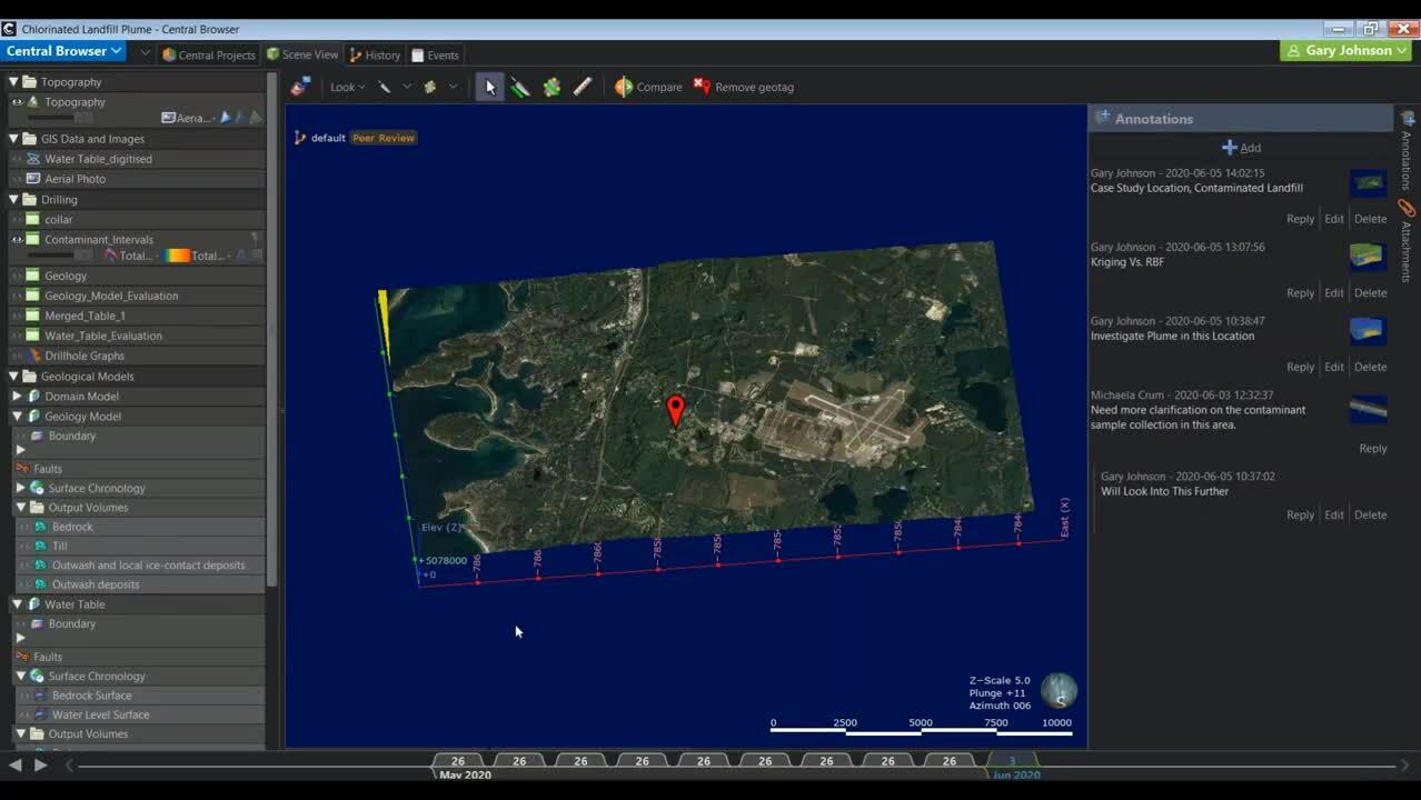
The interface that you are seeing now

[00:08:16.000]
is the Central browser.

[00:08:18.230]
Now, as I mentioned, Seequent Central

[00:08:20.030]
is our cloud-based model management

[00:08:21.750]
and collaboration solution.

[00:08:24.340]
For contaminated sites,

[00:08:27.060]
there’s always oversight involved,

[00:08:29.210]
whether it’s through stakeholders

[00:08:31.000]
and/or your project managers.

[00:08:33.800]
Of course, there’s not normally a single person

[00:08:36.440]
working on this project and it is a collaborative effort

[00:08:40.400]
through multiple individuals.

[00:08:42.770]
Now, one of the huge benefits

[00:08:45.910]
of 3D modeling and visualization

[00:08:48.610]
is the ability to communicate

[00:08:51.170]
to everyone involved in the project.

[00:08:53.670]
Everyone from regulators to your colleagues

[00:08:56.520]
that might be assisting you in building the model.

[00:09:00.120]
Seequent Central allows you to track

[00:09:03.080]
a project’s history through time,

[00:09:05.360]
but it also allows you to create annotations and communicate

[00:09:10.330]
allowing for a clear and visible QA/QC process.

[00:09:14.920]
Now, within the interface we have here our case study,

[00:09:19.580]
a contaminated landfill site.

[00:09:22.610]
This is publicly available data by the way.

[00:09:27.080]
The Central browser allows you to, of course,

[00:09:29.300]
interact with objects in 3D,

[00:09:31.890]
but it also allows you, over here on the right,

[00:09:34.830]
to actually comment and make annotations.

[00:09:38.540]
Now, this allows you to have multiple colleagues

[00:09:42.900]
and/or stakeholders to have insight into the project

[00:09:46.817]
and to communicate in real-time.

[00:09:49.040]
Here, I’ve made a few simple notes

[00:09:50.920]
with some geotags as well,

[00:09:53.930]
and so has one of my colleagues, Michaela.

[00:09:56.670]
And we can actually respond directly

[00:09:59.040]
to each other’s comments,

[00:10:00.760]
whether this is used to actually highlight

[00:10:02.690]
the contaminant plume,

[00:10:04.100]
or in the case of Michaela’s comment here,

[00:10:07.150]
she actually highlighted an area where we thought

[00:10:09.700]
that we might need some more samples collected.

[00:10:12.770]
Now this is great for QA/QC process,

[00:10:15.450]
or if your colleagues just have questions

[00:10:17.650]
or want visibility into the project.

[00:10:22.650]
The Central browser allows anyone

[00:10:25.910]
that needs insight into the project

[00:10:27.900]
to be able to access that.

[00:10:29.920]
Now it’s important to mention

[00:10:32.470]
that you have complete control over your own Central,

[00:10:36.680]
your Central server,

[00:10:38.760]
and so you can grant individuals access to this

[00:10:42.340]
and control their permissions.

[00:10:43.900]
For example, you might only want them

[00:10:45.600]
to be able to view the data,

[00:10:47.830]
you might want them to be able to make comments

[00:10:49.770]
and annotations,

[00:10:50.970]
and you might want to revoke access at any time,

[00:10:53.870]
and you can do so with your own Central browser.

[00:10:57.620]
Now, this is a great model management

[00:11:00.510]
and collaboration solution,

[00:11:01.770]
but it’s not where you’re actually building the model.

[00:11:04.490]
And this is not where the actual Contaminants extension

[00:11:07.340]
is stored,

[00:11:08.520]
but I thought that it’s really important to mention

[00:11:11.330]
that the Central browser is great for contaminated sites,

[00:11:15.730]
because it allows you to track the plume through time

[00:11:18.790]
and to track the overall project through time.

[00:11:22.230]
And most contaminated sites are long-term projects,

[00:11:26.500]
which involve remediation, and of course,

[00:11:30.590]
a changing contaminant plume

[00:11:33.380]
through the project’s life cycle.

[00:11:36.640]
I will now jump into Leapfrog Works

[00:11:39.590]
and to actually demonstrate

[00:11:41.600]
the capabilities of the Contaminants extension.

[00:11:46.910]
Here I will start by actually introducing the project site.

[00:11:51.680]
Now I have already mentioned

[00:11:52.850]
this is a contaminated landfill,

[00:11:56.210]
and here is some of the data

[00:11:58.040]
that was actually originally collected for this project.

[00:12:01.720]
We have some contaminated screens

[00:12:04.020]
with total chlorine concentrations,

[00:12:06.550]
and we have a topography and map representing the site area,

[00:12:11.110]
just to give you some reference

[00:12:12.380]
into what we’re actually dealing with.

[00:12:14.710]
Now, this is a coastal site,

[00:12:18.000]
and this data is publicly available and included

[00:12:22.090]
in our online training for the Contaminants extension.

[00:12:26.660]
The Contaminants extension in Leapfrog Works

[00:12:29.560]
is very similar to the Hydrogeology extension,

[00:12:33.107]
and that it gives you access to an additional folder

[00:12:36.290]
in the project tree.

[00:12:38.210]
The project tree in Leapfrog Works is designed

[00:12:40.830]
in a top-down approach,

[00:12:42.380]
which is designed to match your workflow,

[00:12:45.370]
and the Contaminants extension actually now

[00:12:48.320]
gives you access to the contaminant models folder,

[00:12:51.320]
which you can see over here on the left in the project tree.

[00:12:56.020]
The contaminant models folder is

[00:12:59.830]
also designed in a workflow orientated solution,

[00:13:03.270]
where you’re first going to be setting up your estimations,

[00:13:06.370]
which you can see here contained in your estimation folder.

[00:13:10.320]
You will then be designating your domain,

[00:13:14.770]
designating the values that you want to use

[00:13:17.170]
within your domain.

[00:13:18.560]
In this case study,

[00:13:19.690]
we’ll actually only be considering

[00:13:21.790]
the unconsolidated material above the bedrock.

[00:13:26.150]
You will then establish your spatial models

[00:13:29.520]
where you actually have control over the variography,

[00:13:32.800]
in both 2D and 3D.

[00:13:35.470]
You’ll be setting up your variable orientations,

[00:13:38.130]
which can allow you to account

[00:13:39.970]
for a multitude of different surfaces,

[00:13:42.900]
whether it’s geologic surfaces and/or a water table

[00:13:46.430]
and so on.

[00:13:48.520]
And then we actually give you access

[00:13:50.800]
to multiple different estimators,

[00:13:52.960]
and/or interpolation methods

[00:13:55.220]
within Leapfrog Works with the Contaminants extension.

[00:13:59.010]
Now, this is something that has been asked for

[00:14:01.730]
throughout Leapfrog’s life cycle,

[00:14:04.690]
and with the Contaminants extension,

[00:14:06.730]
you now have access to use,

[00:14:08.550]
not just the standard radial basis function or RBF,

[00:14:12.560]
which is used in creating numeric models in Leapfrog,

[00:14:15.980]
but we also have access to a new inverse distance estimator,

[00:14:20.690]
new nearest neighbor estimator, and kriging.

[00:14:26.720]
In addition to kriging,

[00:14:27.930]
we have ordinary and simple kriging estimation methods

[00:14:32.160]
available within the Contaminants extension.

[00:14:36.320]
Now, once you have set up your estimators,

[00:14:39.070]
and/or used your estimators

[00:14:41.120]
within the Contaminants extension,

[00:14:43.240]
the Contaminants extension gives you access

[00:14:45.440]
to create block models to actually go through

[00:14:48.720]
and visualize that data in 3D.

[00:14:54.010]
Block models also give you the ability

[00:14:56.840]
to create calculations and filters and generate reports

[00:15:01.410]
based on those calculations that you have scripted

[00:15:04.070]
within the Leapfrog interface.

[00:15:07.760]
Because this is a workflow-orientated solution,

[00:15:10.480]
I will now actually walk you through

[00:15:12.770]
the basic workflow of using the Contaminants extension

[00:15:16.390]
within Leapfrog Works.

[00:15:19.660]
The first scene I have here is, of course,

[00:15:22.450]
of the case study site.

[00:15:25.960]
Now this was the data that was actually collected for this,

[00:15:29.340]
and you can see, we have quite a bit of contaminant data.

[00:15:32.810]
This is all chlorine concentrations.

[00:15:35.640]
The first step in the process is to set up a new estimation

[00:15:39.880]
in the Leapfrog’s contaminants models folder.

[00:15:43.720]
This can be done by just right clicking

[00:15:45.180]
on the estimation folder

[00:15:46.400]
and setting up a new contaminant estimation.

[00:15:50.290]
What you’ll then do

[00:15:51.170]
is you will actually set up the domain

[00:15:53.320]
that you want to estimate within.

[00:15:55.830]
The visual that you can see here is showing you

[00:15:58.660]
that all of our contaminant data is actually collected

[00:16:02.870]
in the unconsolidated sediments above the bedrock,

[00:16:07.600]
and the bedrock here is actually this green lithologic unit.

[00:16:13.210]
Because we can actually designate a domain

[00:16:15.760]
to estimate within,

[00:16:16.870]
we can only consider the relevant lithologic unit.

[00:16:22.280]
Now, this can be above or below a water table.

[00:16:26.410]
You can use multiple different parameters

[00:16:28.400]
to actually set up your domain, but in this instance,

[00:16:31.150]
we’re just using unconsolidated material.

[00:16:34.800]
With the domain,

[00:16:36.940]
you now have the ability to set a hard or soft boundary.

[00:16:42.280]
A hard boundary will only consider data points

[00:16:45.070]
within the domain you have set up,

[00:16:46.560]
for example, the unconsolidated sediments,

[00:16:48.787]
and a soft boundary allows you to actually consider data

[00:16:52.850]
within a certain designated range of that domain.

[00:16:58.210]
So for example, if I wanted to estimate data within 25 units

[00:17:02.730]
of the unconsolidated sediments,

[00:17:04.630]
I would use a soft boundary.

[00:17:09.660]
The next step in the process

[00:17:10.920]
after you have actually set up your domain,

[00:17:13.410]
is to actually create your spatial models.

[00:17:19.200]
The spatial models in Leapfrog

[00:17:21.860]
allow you to orientate the ellipsoid in 3D,

[00:17:26.580]
but you also have control over the variography

[00:17:29.310]
in 2D as well.

[00:17:30.410]
So the ellipsoid that you see here,

[00:17:33.430]
is actually corresponding to the settings

[00:17:36.180]
that have been established in the experimental variograms,

[00:17:40.470]
which can be all controlled in this interface,

[00:17:43.640]
in two dimensions.

[00:17:45.270]
You can of course control the radial plot,

[00:17:47.400]
but you can also control the major, semi-major,

[00:17:51.230]
and minor axes,

[00:17:54.860]
giving you complete control over the variography

[00:17:59.690]
of this estimation.

[00:18:03.070]
Now, once you’ve set up your ellipsoid,

[00:18:05.230]
and this can, of course,

[00:18:06.063]
also be done in two dimensions as well,

[00:18:10.470]
you’ll actually want to go in it

[00:18:12.050]
and create your different estimators.

[00:18:16.710]
Now, this is where we have added

[00:18:18.160]
quite a bit of functionality to Leapfrog in that,

[00:18:21.290]
you can now use multiple different estimation methods

[00:18:24.910]
or interpolation methods.

[00:18:27.410]
And then once you have set these up,

[00:18:29.200]
you can actually evaluate the estimators onto a block model.

[00:18:35.650]
Block models are great for visualization purposes

[00:18:38.160]
and/or if you’re creating a cross section.

[00:18:42.300]
Here, we can actually visualize

[00:18:43.660]
not just the domain geologic model,

[00:18:47.000]
we can visualize our kriging estimation,

[00:18:50.490]
we can visualize our RBF estimation,

[00:18:53.640]
and we can compare and contrast the differences,

[00:18:56.390]
but we can also create different calculations.

[00:19:00.450]
For example, we have a confidence calculation of our plumes

[00:19:03.230]
that we can now visualize.

[00:19:06.920]
Here, we can see the different confidence levels,

[00:19:08.800]
which we have designated of our contaminant plume

[00:19:11.640]
and to data gathered for this project.

[00:19:15.190]
Now, these calculations are completely up to you.

[00:19:20.810]
You now have the ability to script calculations

[00:19:23.410]
within Leapfrog.

[00:19:25.130]
So I will show you what the scripting interface looks like,

[00:19:28.600]
and if you have scripted in the past, for example, in Excel,

[00:19:31.870]
most of these logic statements and/or variables

[00:19:35.120]
will look familiar to you.

[00:19:37.040]
We’ve tried to design the Contaminants extension in

[00:19:43.180]
an approach that can be of course, easy to learn,

[00:19:46.460]
but also auditable.

[00:19:47.800]
It’s not split meant to the black box,

[00:19:49.750]
you’re meant to have complete control over

[00:19:51.580]
not just the actual estimators being used,

[00:19:54.850]
but also the calculations and scripts

[00:19:56.930]
that go in to your reporting methods.

[00:20:02.010]
These are meant to be defensible calculations,

[00:20:04.990]
so you now have complete control over them.

[00:20:07.840]
And we want to democratize the ability

[00:20:11.130]
to actually estimate contaminants

[00:20:14.020]
and create contaminant plumes.

[00:20:17.320]
Now, these scripts

[00:20:21.270]
actually utilize very common logic statements,

[00:20:23.680]
such as if then statements,

[00:20:25.430]
but there is a lot that you can do here.

[00:20:27.150]
You can actually create mathematical calculations.

[00:20:30.610]
For example, porosity and permeability

[00:20:33.240]
can all be factored into these calculations.

[00:20:37.130]
And these can then be visualized on the block model,

[00:20:42.260]
or you can actually create reports.

[00:20:44.330]
So I’m going to open up what we call a contaminant report

[00:20:47.070]
in Leapfrog.

[00:20:50.170]
This contaminant report actually utilizes

[00:20:53.490]
both category columns and value columns.

[00:20:58.040]
Now these category columns and value columns

[00:21:01.060]
actually include, of course, the geologic models,

[00:21:04.330]
as well as the estimators and calculations

[00:21:07.700]
that you have scripted within the Leapfrog interface.

[00:21:11.670]
This can allow you to determine contaminant mass

[00:21:14.300]
while setting up multiple different cutoff levels

[00:21:17.140]
for a contaminant,

[00:21:19.050]
and this can be key for reporting methods,

[00:21:21.540]
so this can be included as a PDF document,

[00:21:24.780]
but it can also be used for actual calculations

[00:21:28.920]
of mathematical properties of the contaminants

[00:21:32.590]
in the ground.

[00:21:33.840]
And this is meant to be intuitive and easy to learn,

[00:21:38.420]
as the key things to note,

[00:21:39.910]
and we do not want you to have to have a single gatekeeper

[00:21:45.420]
of the Leapfrog Contaminants extension.

[00:21:48.310]
We want this to be readily available to anyone

[00:21:50.960]
who wants to learn 3D modeling in the contaminant realm.

[00:21:59.270]
So I’m going to jump back into Leapfrog.

[00:22:02.420]
I’m going to show a little tips and tricks.

[00:22:04.650]
I’m going to collapse the project tree.

[00:22:08.860]
And once again, the Contaminants extension

[00:22:11.190]
will give you access to the contaminants models folder,

[00:22:15.850]
which is a new and exciting tool in Leapfrog Works.

[00:22:21.700]
Now, we are currently offering free trials

[00:22:24.620]
of both the Contaminants extension and Seequent Central,

[00:22:27.750]
our model management and collaboration solution.

[00:22:31.620]
If you are interested in the Contaminants extension,

[00:22:34.090]
don’t hesitate to reach out

[00:22:35.440]
to your personal account manager,

[00:22:37.420]
and/or contact one of our local sales representatives

[00:22:40.350]
at [email protected].

[00:22:44.140]
For workflow and technical support,

[00:22:46.470]
contact our team at [email protected].

[00:22:50.600]
Important to mention that our support is free

[00:22:53.290]
and included with all commercial and trial options,

[00:22:56.540]
so don’t hesitate to take advantage of that.

[00:23:00.280]
And for all other questions,

[00:23:02.140]
please visit our website at seequent.com.

[00:23:04.550]
We now have free online training

[00:23:06.880]
for the Contaminants extension.

[00:23:08.900]
So if you are not familiar with using Leapfrog,

[00:23:11.210]
we have free training available to you,

[00:23:13.470]
and we want you to take advantage of that as well.

[00:23:17.690]
<v ->Thank you, Thomas and Gary.</v>

[00:23:19.549]
And thank you everyone for attending today’s webinar.

[00:23:22.536]
If you have any other questions,

[00:23:24.150]
please contact our technical support team

[00:23:26.170]
at [email protected].

[00:23:29.800]
On behalf of Seequent,

[00:23:31.040]
thank you for joining us and have a great rest of your day.