GeoStudio Core: Integrating SLOPE/W, SEEP/W, and SIGMA/W to solve more complex problems

This video will take you through the step-by-step process of defining the analysis tree, materials, and geometry, followed by reviewing the results of an example project.

The GeoStudio Core bundle combines the three GeoStudio products that are most commonly used in engineering projects: SLOPE/W, SEEP/W and SIGMA/W. The integration of these three products can help you achieve realistic results for various real-world problems.

Overview

Video Transcript

[00:00:03.540]
<v Vincent>Hello, and welcome to this GeoStudio Tech Talk.</v>

[00:00:06.720]
These monthly webinars are designed to improve

[00:00:08.880]
understanding of the software

[00:00:10.610]
and ultimately promote success in engineering projects.

[00:00:14.350]
This month’s Tech Talk will feature GeoStudio Core

[00:00:17.810]
integrating SLOPE/W, SEEP/W, and SIGMA/W

[00:00:21.820]
to solve complex problems.

[00:00:24.860]
I’m Vincent Castonguay.

[00:00:26.610]
I work as a research and development specialist

[00:00:28.880]
with the GeoStudio Business Unit here at Seequent.

[00:00:32.620]
Today’s webinars will be approximately 60 minutes long.

[00:00:36.220]
Attendees can ask questions using the chat feature.

[00:00:39.920]
I will respond to these questions via email

[00:00:42.170]
as quickly as possible, and a recording of the webinar

[00:00:45.960]
will be available so participants can review

[00:00:48.300]
the demonstration at a later time.

[00:00:51.679]
GeoStudio is a software package

[00:00:53.270]
developed for a geotechnical engineers

[00:00:55.240]
and earth scientists comprising several products.

[00:00:58.630]
The range of products allows users

[00:01:01.030]
to solve a wide array of problems

[00:01:02.740]
that may be encountered in these fields.

[00:01:05.390]
Today’s would be in our relates specifically

[00:01:07.410]
to three of our products, SLOPE/W, SEEP/W, AND SIGMA/W.

[00:01:13.690]
Those looking to learn more about the products,

[00:01:15.730]
including background theory, available features,

[00:01:18.370]
and typical modeling scenarios

[00:01:20.580]
can find an extensive library of your sources

[00:01:23.430]
GeoStudio website.

[00:01:26.040]
There you can find tutorial videos,

[00:01:28.040]
examples with detailed explanations

[00:01:30.490]
and engineering books on each product.

[00:01:35.050]
Let me start this webinar by showing you

[00:01:37.050]
this beautiful picture of a slope plunging toward the sea.

[00:01:41.370]
This is either a tourist dream spot

[00:01:43.590]
or the geotechnical engineers nightmare,

[00:01:45.860]
depending on who’s looking at it.

[00:01:49.160]
A geotechnical engineer will naturally see option two.

[00:01:52.170]
This complex, natural geological feature

[00:01:54.660]
will often be turned into a 2D representation

[00:01:57.800]
stripped of as much of the complexities as possible

[00:02:01.160]
to understand the key mechanisms, controlling behavior.

[00:02:05.710]
A question a geotechnical engineer might need to answer

[00:02:08.430]
regarding this slope is, is the slope stable?

[00:02:12.840]
To better represent the problem

[00:02:14.500]
and be able to properly answer the questions

[00:02:16.860]
we might have to consider the water conditions

[00:02:19.210]
that exist in the slope.

[00:02:21.070]
Where’s the water table?

[00:02:22.570]
How does it affect shear resistance?

[00:02:25.520]
We might also need to consider if there are stresses

[00:02:28.880]
and strain conditions that affect the slope as well.

[00:02:33.750]
Once all of these elements are considered,

[00:02:37.180]
then we can begin to answer the engineering question

[00:02:39.830]
and proceed to a slope stability analysis.

[00:02:45.340]
The process I just described

[00:02:46.870]
is exactly what this webinar’s all about.

[00:02:49.890]
How can we use the GeoStudio Core products

[00:02:52.510]
in an integrated way to solve a complex engineering problem?

[00:02:58.970]
In this webinar,

[00:03:00.060]
we will first review the GeoStudio Core products.

[00:03:04.270]
Next, I will spend a moment discussing

[00:03:06.330]
the numerical modeling process

[00:03:08.017]
and the important aspects to consider,

[00:03:10.600]
to conduct a successful numerical analysis.

[00:03:15.300]
Finally, I will demonstrate how to put this on into practice

[00:03:18.400]
by creating an example where the construction sequence

[00:03:21.520]
of two embankment is simulated

[00:03:23.860]
using the full GeoStudio Core lineup of products.

[00:03:31.070]
Let’s dive into it by reviewing each product

[00:03:33.980]
that composes the GeoStudio Core lineup.

[00:03:38.240]
As I mentioned earlier,

[00:03:39.940]
GeoStudio Core refers to the three most popular products

[00:03:43.230]
part of the GeoStudio portfolio.

[00:03:46.620]
SLOPE/W, SEEP/W, and SIGMA/W.

[00:03:51.030]
SLOPE/W is a limit equilibrium stability application,

[00:03:54.870]
where a slope is split into a number of slices,

[00:03:58.100]
driving in resisting forces are calculated

[00:04:00.420]
within each slice,

[00:04:02.490]
and factors of safety are computed.

[00:04:05.120]
Slope is all fundamentally about comparing resistance

[00:04:08.390]
versus driving forces.

[00:04:11.670]
Water seepage is often a governing factor

[00:04:14.290]
in many geotechnical problematics.

[00:04:16.900]
SEEP/W is a finite element software

[00:04:19.470]
where a domain is disguised into small elements

[00:04:23.180]
in order to resolve the water balance within the domain.

[00:04:27.610]
SEEP/W will help establish water conditions

[00:04:29.940]
that can then be used by other modules in GeoStudio.

[00:04:34.980]
Finally, SIGMA/W is the stress-train modeling module

[00:04:38.860]
in GeoStudio.

[00:04:40.832]
Similar to how SEEP/W functions,

[00:04:43.460]
SIGMA/W disguises a domain into finite elements,

[00:04:47.440]
but this time to resolve the force-displacement equilibrium.

[00:04:51.820]
SIGMA/W helps establishing the stresses and strains

[00:04:55.070]
that exist within a domain.

[00:04:59.400]
The strength of the GeoStudio Core package

[00:05:01.840]
lies within the tight implementation

[00:05:03.650]
of the various physics that interact with each other.

[00:05:07.140]
Groundwater conditions calculated with SEEP,

[00:05:09.770]
can be made to influence the stresses and strains

[00:05:12.390]
that are calculated with SIGMA/W.

[00:05:15.130]
Both of these physics can in turn,

[00:05:17.120]
be brought in to SLOPE/W

[00:05:18.620]
to calculate the stability of a slope or earth structure.

[00:05:22.780]
Each model can be made to impact the others in various ways

[00:05:26.320]
that we will discuss in this webinar.

[00:05:30.400]
Let us now focus on the numerical modeling process

[00:05:33.250]
and what are some of the important aspects to consider

[00:05:36.210]
when setting up a more complex numerical analysis.

[00:05:39.970]
Using SEEP/W and SIGMA/W in conjunction with SLOPE/W

[00:05:44.300]
brings some new challenges that need to be addressed,

[00:05:47.670]
especially for users who are more experienced

[00:05:50.200]
with using SLOPE/W alone.

[00:05:54.770]
Imagine I have an engineering problem to solve,

[00:05:57.000]
and I wished to proceed via numerical modeling

[00:05:59.180]
to help me with this task.

[00:06:01.740]
I will first need to conceptualize the problem at hand

[00:06:04.320]
so that I can subject my conceptual model to analysis.

[00:06:08.800]
So for example,

[00:06:09.633]
this slope that I showed at the beginning of the webinar

[00:06:11.910]
could be conceptualized as the following geometry.

[00:06:15.530]
Conceptualization has at its core

[00:06:18.090]
the idea of simplification.

[00:06:20.530]
When performing numerical simulations,

[00:06:22.560]
we tend to over complicate the geometries that we use

[00:06:25.740]
probably in fear of missing out on important details.

[00:06:29.690]
If you go back in mere 10 or 20 years,

[00:06:32.390]
trying to solve very complex geometries

[00:06:34.630]
would have been almost impossible

[00:06:36.050]
because of lack of computational power.

[00:06:38.980]
Nowadays however, the most basic laptops

[00:06:41.530]
can solve quite complex problem.

[00:06:44.410]
So in a way, there’s a tendency to avoid simplifying

[00:06:48.070]
problem geometries

[00:06:48.980]
because we know the computer can handle it.

[00:06:52.120]
But the point remains that simpler geometries

[00:06:54.840]
often lead to easier results interpretation.

[00:06:58.580]
We should thus simplify as much as we can

[00:07:01.450]
and come back later on when we have a good grasp

[00:07:03.830]
on what the results mean

[00:07:05.560]
and add more complexity, if necessary.

[00:07:10.360]
The next step to solve the numerical modeling problem

[00:07:12.700]
would be to carefully choose the physics

[00:07:14.500]
that apply to the problem at hand.

[00:07:16.960]
I like to view these physics

[00:07:18.310]
in terms of GeoStudio products.

[00:07:20.740]
For example, if I’m trying to model

[00:07:22.230]
the effect of disappearing permafrost under a culvert,

[00:07:25.750]
I’ll need to include in my model SEEP/W

[00:07:29.070]
to account for water transfers,

[00:07:31.590]
TEMP/W to simulate the heat exchanges,

[00:07:34.240]
and SIGMA/W to compute the resulting stress-strain behavior.

[00:07:38.680]
Any engineering problem should be carefully studied

[00:07:41.060]
to decide what physics apply into consequently,

[00:07:44.080]
which GeoStudio module should be included in the analysis.

[00:07:50.060]
As we add physics into our models,

[00:07:52.610]
we also need to choose which constitutive laws

[00:07:56.050]
will correctly represent to soil behavior.

[00:07:59.260]
A constitutive law is a set of mathematical equations

[00:08:03.480]
that wishes to translate real soil behavior

[00:08:06.350]
into computer language

[00:08:07.720]
so that GeoStudio can adequately model the soils

[00:08:10.930]
in a way that fits the field reality.

[00:08:14.109]
Constitutive laws exists to represent

[00:08:16.810]
the stress-train behavior of soils, for example,

[00:08:19.090]
or the ability to transfer water and heat

[00:08:22.020]
or any other behavior feature we deem important

[00:08:24.660]
in our simulations.

[00:08:28.050]
Various parts of a domain can require

[00:08:30.240]
distinct constitutive laws

[00:08:32.310]
as the materials might behave quite differently.

[00:08:35.670]
Choosing the appropriate constitutive law

[00:08:37.660]
for a particular soil requires knowledge and experience.

[00:08:41.920]
While it is not necessary to know and understand

[00:08:44.500]
every intricate detail of the workings

[00:08:47.100]
of the various constitutive laws,

[00:08:49.600]
it is important to have a general understanding

[00:08:51.680]
of the models we choose to use.

[00:08:53.350]
Otherwise we might be unable

[00:08:55.060]
to correctly interpret the results.

[00:08:58.810]
The next item on the list to define

[00:09:01.120]
is the boundary conditions that apply to our domain.

[00:09:04.560]
Boundary conditions can take many forms

[00:09:06.440]
depending on what type of analysis we are conducting,

[00:09:09.400]
but they generally serve the same general purpose

[00:09:12.690]
and forcing certain conditions to part of the domain

[00:09:15.910]
in order to drive the simulations.

[00:09:19.380]
In the case of a SIGMA/W simulation, for example,

[00:09:22.180]
boundary conditions could include limiting displacements

[00:09:26.020]
on the edge of the domain or applying forces and stresses.

[00:09:30.880]
Specifying the hydraulic condition

[00:09:33.010]
is also a form of boundary condition application.

[00:09:36.900]
Appropriately defining the boundary conditions

[00:09:39.350]
that apply to a numerical model can be quite challenging

[00:09:42.580]
and might be easy to overlook.

[00:09:45.120]
Specifying the wrong bunch of conditions for a problem

[00:09:48.130]
will cost just as much problem for the overall solution

[00:09:51.160]
as would using a batch geometry

[00:09:53.040]
or failing to choose the appropriate inputs

[00:09:55.700]
for the constitutive laws.

[00:09:59.750]
Once the steps one to four I’ve been properly dealt with,

[00:10:04.120]
we can move on to solve the numerical analysis.

[00:10:06.540]
We call this step, interpretation.

[00:10:10.010]
For the user, this is generally the simpler step

[00:10:12.750]
of the whole modeling process.

[00:10:15.890]
Once the calculations are completed,

[00:10:18.349]
GeoStudio will output results,

[00:10:19.860]
that can be viewed through contour plots

[00:10:21.760]
or line plots for example.

[00:10:24.880]
But calculated results in themselves aren’t worth much

[00:10:28.670]
if they are not properly verified by a competent user.

[00:10:33.340]
This step is crucial in any numerical analysis.

[00:10:37.980]
One must have sufficient knowledge and experience

[00:10:40.470]
to be able to look at simulation results

[00:10:42.830]
and assess if the response

[00:10:44.630]
as computed by the software makes sense.

[00:10:47.750]
In most cases, the software will input some results.

[00:10:51.730]
It is up to the user to understand what these results mean.

[00:10:56.090]
And we often say that the numerical modelers

[00:10:58.090]
should know the answer they expect

[00:10:59.810]
before even launching the software they intent to use.

[00:11:02.920]
Having a general idea of how the results should look

[00:11:07.170]
will help user on interpret

[00:11:09.730]
what the software is telling them.

[00:11:13.790]
Finally, this verification step might reveal some flaws

[00:11:17.330]
and choices made along the way

[00:11:19.280]
from conceptualization to interpretation.

[00:11:22.880]
It is quite common then that we will need

[00:11:25.010]
to take a step back as we inspect computed results

[00:11:28.030]
to rethink our constitutive law choices, for example,

[00:11:31.050]
or that particular boundary condition we were unsure about,

[00:11:35.230]
if it was appropriate or not.

[00:11:37.980]
Critically assessing these choices

[00:11:40.300]
will help produce higher quality numerical simulations.

[00:11:46.690]
A feature of numerical modeling

[00:11:48.050]
that users will most often encounter

[00:11:50.430]
is what we call parent-child relationships.

[00:11:53.680]
In real life a child inherits certain characteristics

[00:11:56.743]
of their parents, which they can in turn pass along

[00:11:59.910]
to their own child.

[00:12:01.610]
Child’s of the same parents

[00:12:03.200]
will share the same characteristics.

[00:12:06.430]
Well, the same holds true for GeoStudio analysis.

[00:12:09.350]
These characters takes parent analysis

[00:12:12.050]
will pass on to child analysis,

[00:12:14.920]
will take the form of stressors, pore-water pressure,

[00:12:17.920]
accumulator strains, and so on.

[00:12:20.360]
This helps create hierarchy and structure

[00:12:22.930]
in complex analysis trees where many analysis types

[00:12:27.590]
might cohabit and share information.

[00:12:30.540]
So for example, in this analysis tree,

[00:12:33.210]
all the analysis displayed share the same geometry.

[00:12:38.120]
The seepage analysis sits one hierarchy level higher

[00:12:41.030]
in the analysis tree than the In-Situ analysis.

[00:12:44.050]
As such, the seepage analysis acts as the parent

[00:12:47.180]
while the In-Situ analysis is the child.

[00:12:49.940]
The In-Situ analysis can then inherits certain features

[00:12:53.070]
of the seepage analysis, in this case,

[00:12:55.410]
pore-water pressure conditions.

[00:12:57.810]
We can define this when defining each analysis.

[00:13:01.960]
Important to note here is the limit equilibrium analysis

[00:13:05.040]
displayed further down in the analysis tree.

[00:13:07.830]
This analysis is also a direct child

[00:13:09.730]
of the seepage analysis.

[00:13:11.770]
Since it sits at the same level as the In-Situ analysis,

[00:13:15.290]
you can call the siblings.

[00:13:17.570]
They both have access to the information

[00:13:19.280]
provided by the parents, seepage analysis.

[00:13:23.290]
Continuing on in the analysis tree,

[00:13:25.580]
the stress correction analysis sits one hierarchy level

[00:13:28.550]
below the In-Situ analysis.

[00:13:31.697]
The In-Situ analysis is then considered

[00:13:34.220]
the parent of the stress correction analysis,

[00:13:36.220]
and it can pass along information to it.

[00:13:39.810]
Finally, that analysis labeled tree, A, B, and C

[00:13:44.330]
are all siblings

[00:13:45.390]
whose parents is the stress correction analysis.

[00:13:51.320]
We are now ready to move on to the practical example

[00:13:54.290]
we will analyze to illustrate the various concepts

[00:13:56.610]
that were discussed in the webinar.

[00:14:00.730]
Cubzac-les-Ponts refers to test embankments

[00:14:03.640]
constructed in the 1980s in France

[00:14:06.200]
and studied by various researchers.

[00:14:09.540]
Two embankments in particular were analyzed.

[00:14:12.060]
Embankment A, which was both built fast and high

[00:14:15.830]
to purposely result in failure of the underlying soft clay.

[00:14:21.470]
Embankment B was constructed slowly

[00:14:24.150]
to monitor how pore-water pressure dissipation

[00:14:26.580]
would occur in the underlying soft clay.

[00:14:31.650]
The goal here is to use GeoStudio Core

[00:14:33.900]
to replicate the results.

[00:14:37.760]
The construction sequence for both embankments

[00:14:40.680]
is shown on this plot.

[00:14:42.850]
Embankment A, shown in blue was constructed in four lifts

[00:14:46.640]
and reached a maximum height of 4.5 meters

[00:14:49.260]
after eight days of construction.

[00:14:51.820]
Embarkment B, shown in red was constructed in six lifts

[00:14:55.340]
and only reached a maximum height of 2.4 meters

[00:14:58.080]
after six days of construction.

[00:15:00.790]
Embankment A failed on the ninth day

[00:15:02.960]
while Embankment B was monitored for years

[00:15:05.230]
after construction stopped.

[00:15:08.360]
Here is a cross section of embankment A

[00:15:10.420]
where we can see the four lifts of feel in orange,

[00:15:13.490]
built on top of a two-meter thick desiccated crust

[00:15:17.020]
in yellow.

[00:15:18.980]
And the rest of the soil deposit

[00:15:20.540]
is a soft clay material in green.

[00:15:24.820]
Similarly, here is embankment B’s geometry,

[00:15:27.830]
where we can see a smaller total height for the embankment,

[00:15:31.480]
as well as the small lifts used.

[00:15:34.540]
Since both embankments were constructed on the same site,

[00:15:38.610]
we encountered a same desiccated, crust

[00:15:40.810]
and soft clay deposits.

[00:15:43.290]
To cut computational effort in half,

[00:15:45.540]
we can make use of the symmetry of the geometry

[00:15:47.790]
by cutting the domain in half

[00:15:49.300]
where the summitry axis passes.

[00:15:52.340]
We will see later how boundary conditions

[00:15:54.280]
where that symmetry axis lies need to be modified

[00:15:57.330]
to properly account for the simplification.

[00:16:02.040]
The initial hydraulic conditions

[00:16:03.560]
are very simple at the test site

[00:16:05.320]
with the frantic surface being positioned

[00:16:07.510]
at eight meter of elevation,

[00:16:09.150]
midway into that desiccated crust.

[00:16:11.770]
These conditions apply to both embankments.

[00:16:16.530]
Let us now take a look at the analysis tree structure

[00:16:19.250]
for each embankment scenario.

[00:16:21.790]
For embankment A, the first analysis performed

[00:16:24.340]
uses SEEP/W to calculate the pore-water pressure

[00:16:27.090]
in the domain.

[00:16:28.840]
Next, a SIGMA/W In-Situ analysis is performed

[00:16:32.260]
to initiate the stress conditions within the domain.

[00:16:36.930]
Note here the father child relationship.

[00:16:39.280]
The In-Situ analysis will use a pore-water pressure

[00:16:42.020]
defined by the SEEP/W analysis.

[00:16:44.900]
Next embankment is constructed using SIGMA/W

[00:16:48.093]
consolidation analysis

[00:16:50.130]
following the sequence described earlier.

[00:16:53.160]
The consolidation analysis take advantage of SIGMA/W’s

[00:16:56.370]
fully coupled formulation

[00:16:57.680]
where a pore-water pressure migration

[00:16:59.880]
is properly simulated as soil consolidation occurs.

[00:17:04.490]
The final step to this analysis tree

[00:17:07.030]
is a stress-based stability performed in SLOPE/W.

[00:17:11.230]
The stresses and pore-water pressure conditions

[00:17:13.560]
that exist at the end of stage four of construction sequence

[00:17:17.270]
are passed along to the SLOPE/W analysis

[00:17:22.100]
to calculate the factor of safety.

[00:17:25.889]
A very similar approach is used for embankment B

[00:17:29.660]
where initial pore-water pressures

[00:17:31.687]
are calculated in SEEP/W,

[00:17:34.030]
In-Situ stresses are defined in SIGMA/W,

[00:17:36.390]
and the embankment’s constructioned

[00:17:38.730]
following the slower-paced sequence laid out earlier.

[00:17:42.560]
Once the embankment reaches its maximum height,

[00:17:45.650]
at dissipation phase is performed.

[00:17:48.870]
And essence, this is just a SIGMA/W conciliation analysis

[00:17:52.580]
where no extra load is added

[00:17:54.170]
and where we allow the accessible water pressures

[00:17:57.290]
to dissipate as time passes.

[00:17:59.770]
In this case, the dissipation is allowed to proceed

[00:18:02.250]
during 2000 days, which is roughly five and something years.

[00:18:07.550]
Finally, a stress-based stability analysis is performed

[00:18:11.060]
to verify the factor of safety exactly after

[00:18:15.340]
the six stage of construction.

[00:18:20.440]
The final aspect of these simulations

[00:18:22.430]
that need to be discussed before we jump into GeoStudio

[00:18:25.080]
is material definitions

[00:18:27.320]
or the choices of constitutive laws if you will.

[00:18:31.410]
We will review these choices for each GeoStudio model

[00:18:34.640]
in their respective order of appearance

[00:18:36.530]
in the analysis tree.

[00:18:38.370]
Note that both simulated embankments

[00:18:40.500]
share the exact same soil properties.

[00:18:43.310]
For the SEEP/W analysis,

[00:18:45.640]
the embankment fill is model using a saturated only model

[00:18:49.030]
with a large saturated hydraulic conductivity

[00:18:52.360]
to promote drainage.

[00:18:54.380]
The soft clay is also modeled

[00:18:56.290]
using the saturated only model

[00:18:58.090]
since we expect this material to remain saturated

[00:19:00.590]
throughout the duration of the analysis.

[00:19:03.650]
As you will see a few minutes,

[00:19:05.000]
the desiccated crust must employ

[00:19:06.720]
a saturated/unsaturated model,

[00:19:09.050]
as the water table will fluctuate within this layer

[00:19:12.450]
during the analysis.

[00:19:15.681]
For the SIGMA/W analysis, isotropic elastic materials

[00:19:19.560]
are used for both the embankment fill

[00:19:21.560]
and desiccated crust as these are quite stiff materials,

[00:19:25.410]
and we expect most of the deformations

[00:19:27.310]
to occur in the underlying soft clay.

[00:19:30.580]
The soft clay is modeled

[00:19:31.540]
using the modified cam clay material model.

[00:19:34.490]
This constitutive model

[00:19:35.860]
is formulated on the classical elastic plastic framework

[00:19:39.330]
and exhibits hardening or softening behavior,

[00:19:42.280]
depending on the over consolidations state.

[00:19:45.560]
Moderately over constellated to normally compressed soils

[00:19:48.860]
therefore exhibit accessible water pressures

[00:19:51.690]
due to tendency for both elastic

[00:19:53.880]
and plastic volumetrics training,

[00:19:56.120]
which is an important aspect of soft clay behavior.

[00:20:00.470]
Finally, for the SLOPE/W analysis,

[00:20:03.010]
Mohr-Coulomb material models are used

[00:20:05.060]
so that factors of safety can be calculated

[00:20:07.860]
based on the available resistance

[00:20:09.500]
defined by the Mohr-Coulomb criteria.

[00:20:14.860]
We are in are ready

[00:20:15.693]
for the demonstration part of this webinar.

[00:20:18.610]
I will open GeoStudio

[00:20:20.700]
and walk you through the process of defining and solving

[00:20:23.600]
the values analysis required

[00:20:25.150]
to study the Cubzac-les-Ponts example.

[00:20:30.410]
Here I am in GeoStudio.

[00:20:32.750]
The first step to any new project is to create a new file.

[00:20:36.800]
Let’s choose to metric letter template

[00:20:39.260]
and name the analysis, Cubzac-les-Ponts embankments.

[00:20:44.180]
I’m going to add a first 2D geometry to the project,

[00:20:49.070]
which will be dedicated to embankment A.

[00:20:52.090]
As the geometry will be shared through the values analysis,

[00:20:56.410]
I can define it even before I add

[00:20:58.490]
any specific analysis to the project.

[00:21:01.760]
To make sure I properly track the changes I make,

[00:21:04.700]
I will save the file right away.

[00:21:08.410]
There are many ways to draw a geometry in GeoStudio.

[00:21:11.790]
I already have an Excel workbook

[00:21:13.520]
where the coordinates of the geometry points are listed.

[00:21:17.340]
I will simply copy paste the X and Y columns

[00:21:19.860]
into the defined points window to save time.

[00:21:23.680]
Once this is done,

[00:21:25.350]
all the points needed to draw the geometry are available

[00:21:28.170]
to help me draw the regions

[00:21:29.670]
that will define the various materials

[00:21:31.330]
and highlight the construction sequence.

[00:21:34.290]
By clicking on Draw Regions,

[00:21:36.750]
I can easily draw the lower region where the soft clay lies.

[00:21:46.720]
Then the upper region where the desiccated crust is.

[00:21:49.990]
And finally, each of the four lifts

[00:21:52.890]
used to construct the embankment.

[00:21:56.590]
It is important here that I split the embankment

[00:21:58.840]
into the correct number of lifts,

[00:22:00.850]
even if they will share the same material properties

[00:22:03.900]
as they will be activated or built, if you will,

[00:22:06.540]
in Seequence.

[00:22:09.270]
With the geometry now defined,

[00:22:11.210]
I can go ahead and add a SEEP/W steady-state analysis

[00:22:14.840]
by clicking on Defined Project, then add,

[00:22:18.200]
and finally choosing the steady state option

[00:22:20.810]
within SEEP/W analysis.

[00:22:24.410]
Note that I could change the analysis type to transient

[00:22:28.170]
if I wanted to, later on through this menu.

[00:22:31.660]
I will name this analysis, initial pore-water pressures.

[00:22:37.310]
I will take care of meshing right away

[00:22:39.760]
by clicking on the drum mesh properties button.

[00:22:43.030]
I can change their mesh layout for the whole analysis

[00:22:45.690]
by selecting the entire geometry,

[00:22:48.330]
choosing to edit the selected regions

[00:22:50.650]
and choosing an appropriate meshing pattern.

[00:22:54.030]
Quads and triangle finite elements

[00:22:55.880]
are generally a good choice for most use cases.

[00:22:59.550]
In the Elements tab, I will apply secondary nodes

[00:23:02.720]
as this will provide enhanced precision

[00:23:04.680]
for the SIGMA/W analysis to come.

[00:23:08.110]
Keep in mind that just as for the general geometry

[00:23:11.350]
that is drawn, mission priorities

[00:23:13.410]
will also be shared across all the finite element analysis

[00:23:17.600]
that use a common geometry.

[00:23:20.375]
Given the dimensions of the geometry,

[00:23:22.390]
I will specify a global finite element mesh size

[00:23:25.410]
of one meter.

[00:23:28.400]
I can now inspect the meshing

[00:23:29.710]
to make sure it is appropriate.

[00:23:32.410]
Given the triangular shape of the embankment,

[00:23:34.870]
I could decide to apply triangular elements

[00:23:37.410]
only to this part of the geometry.

[00:23:40.490]
I’m happy with how the meshing looks now.

[00:23:44.480]
As I mentioned earlier,

[00:23:45.670]
when discussing the numerical modeling process,

[00:23:48.470]
once the simple geometry has been defined,

[00:23:51.380]
labeled conceptualization earlier,

[00:23:53.940]
and the proper physics have been chosen, in this case,

[00:23:57.450]
as steady-state seepage analysis,

[00:24:00.020]
I should choose and define the appropriate constitutive laws

[00:24:04.860]
for the problem at hand.

[00:24:07.020]
To do so, I will go into Define Menu and choose materials.

[00:24:12.320]
Let me first define the material properties

[00:24:14.150]
for the desiccated crust.

[00:24:16.400]
The zone of the analysis with the feature both saturated

[00:24:19.670]
and unsaturated flow,

[00:24:21.460]
as the free attic surface will pass through it.

[00:24:24.220]
And water will seep through it

[00:24:26.560]
as the underlying clay consolidates

[00:24:28.810]
because of the weight added by the embankment construction.

[00:24:32.820]
For these reasons, we will use a saturated/unsaturated

[00:24:36.230]
material model here.

[00:24:39.190]
This particular model requires two input functions

[00:24:42.050]
to calculate water flow, the volumetric water content

[00:24:46.200]
and the hydraulic conductivity function.

[00:24:49.950]
Both of these parameters will vary

[00:24:51.410]
as a function of the matrix suction that develops into soil

[00:24:54.610]
as unsaturated flow settles in.

[00:24:58.300]
By clicking on the ellipses on the right,

[00:25:00.820]
I can define each of these functions.

[00:25:03.690]
I will add a new function and use a data point function,

[00:25:08.000]
which allows me to estimate

[00:25:09.370]
the volumetric water content function

[00:25:12.193]
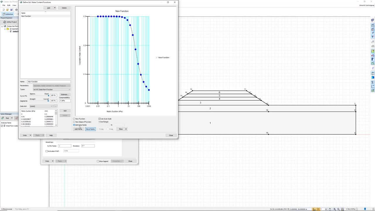
using SEEP/W’s built in simple functions.

[00:25:16.330]
In the case of this desiccated crust,

[00:25:18.780]
the saturated water content is 0.3

[00:25:22.072]
and the material is classified as a silty clay.

[00:25:26.400]
By clicking edit data points,

[00:25:28.600]
I can view the function in semi log space

[00:25:31.180]
and inspect how the volumetric water content

[00:25:33.840]
will vary as a function of matrix suction.

[00:25:37.470]
As suction increases, water is drawn out of the soil,

[00:25:41.690]
and the volumetric water content decreases.

[00:25:45.230]
I’m satisfied with this function and name it crust.

[00:25:49.430]
I finally choose this newly defined function

[00:25:52.480]
through the drop down menu.

[00:25:56.160]
In a similar way,

[00:25:57.700]
I will not create a hydraulic conductivity function

[00:26:00.710]
by clicking on the ellipses on the right

[00:26:02.970]
and choose a data point function type.

[00:26:06.360]
Again, by clicking on estimate,

[00:26:08.310]
I can use SEEP/W’s estimation functions,

[00:26:11.400]
which are quite handy,

[00:26:16.225]
as we don’t necessarily always have access

[00:26:17.790]
to proper laboratory test to define these input functions.

[00:26:22.290]
In this case, I will use the Van Genuchten method

[00:26:25.300]
and associated with the volumetric water content function

[00:26:28.500]
we just defined.

[00:26:30.610]
In the case of the crust, a saturated hydraulic conductivity

[00:26:34.530]
of 0.008 meter per day is suggested

[00:26:38.990]
by the original authors of the Cubzac-les-Ponts study.

[00:26:43.210]
The residual water content is 0.05

[00:26:46.617]
and a maximum suction of a hundred KPA is sufficient here,

[00:26:50.870]
given the small scale of the geometry.

[00:26:54.400]
Inspecting the hydraulic conductivity function generated

[00:26:58.730]
reveals that as metric suction increases

[00:27:02.980]
the hydraulic conductivity decreases,

[00:27:05.180]
which is what we desired.

[00:27:07.770]
I’m satisfied with this function and name it crust.

[00:27:10.670]
And finally, I choose this newly defined function

[00:27:13.530]
through the drop down menu.

[00:27:15.930]
The definition of the material model

[00:27:17.440]
for the desiccated crust is now completed.

[00:27:21.680]
I will add another material,

[00:27:23.830]
this time defining the underlying soft clay.

[00:27:27.400]
As mentioned earlier, since we expect this layer

[00:27:29.960]
to remain fully saturated throughout the analysis,

[00:27:33.120]
we can use the simple saturated only, maternal model.

[00:27:37.540]
The saturated hydraulic conductivity

[00:27:39.560]
is set at 0.001 meter per day.

[00:27:44.840]
And the associated saturated volumetric water content

[00:27:48.230]
is 0.3.

[00:27:51.440]
Finally, the embankment fill material

[00:27:53.730]
is also submitted using a saturated only material model

[00:27:56.930]
for simplicity.

[00:27:58.620]
We use a very high saturated hydraulic conductivity

[00:28:01.180]
of one meter per day to promote fast drainage

[00:28:03.680]
towards the lower parts of the analysis.

[00:28:07.320]
The saturated volumetric water content is 0.4.

[00:28:12.070]
Now that all the materials have been defined,

[00:28:15.030]
I can draw them over the various regions of the geometry,

[00:28:18.040]
starting from the bottom to soft clay,

[00:28:20.750]
then desiccated crust.

[00:28:23.670]
Notice here that I won’t assign the fill material just yet,

[00:28:26.800]
as the goal of this first analysis

[00:28:28.790]
is simply to establish the hydraulic conditions in the soil

[00:28:32.400]
prior to beginning the embarkment construction.

[00:28:37.920]
The last step to perform

[00:28:39.110]
before we can move on to solving the analysis

[00:28:41.500]
is to define appropriate boundary conditions.

[00:28:44.610]
In this case,

[00:28:45.443]
the boundary conditions are very straightforward.

[00:28:47.500]
As the piezometric level was measured

[00:28:49.690]
at eight meter of elevation throughout the site.

[00:28:53.520]
To represent this, I would go into the Define menu

[00:28:56.230]
and choose Boundary conditions.

[00:28:58.530]
I will add a new hydraulic boundary condition,

[00:29:01.640]
choose the water total headkind,

[00:29:04.950]
and define it as a constant head elevation of eight meters.

[00:29:10.060]
I can then name this new boundary condition

[00:29:12.150]
and assign it in an easy two-spot color.

[00:29:24.040]
Once the boundary condition has been created,

[00:29:26.070]
I can click on Draw Boundary Conditions

[00:29:28.700]
or use the dropdown menu

[00:29:30.890]
to apply it to the base of the geometry.

[00:29:33.640]
This means that a total head of eight meters

[00:29:36.410]
will be applied to each of the point

[00:29:38.230]
at the bottom of the analysis.

[00:29:40.770]
When launched calculations,

[00:29:43.400]
SEEP/W will calculate the corresponding pore-water pressures

[00:29:46.820]
everywhere in the domain

[00:29:47.860]
as to satisfy the supply boundary condition.

[00:29:52.220]
We are now ready to solve the analysis.

[00:29:55.550]
Clicking on Start will automatically save the file

[00:29:59.250]
and launch the calculations.

[00:30:01.450]
Once the analysis is marked as solved,

[00:30:04.250]
I can switch to the results view

[00:30:06.090]
and inspect the calculated results.

[00:30:08.230]
This is the all-important verification step

[00:30:10.850]
I alluded to earlier.

[00:30:14.260]
By clicking on Draw ISO Surface,

[00:30:16.060]
I can draw a continuous line

[00:30:17.780]
indicating where water pressure of zero KPA

[00:30:21.950]
is in the domain.

[00:30:23.480]
This is an easy way

[00:30:24.470]
to view where the water table is positioned.

[00:30:27.550]
In this case, as we desired,

[00:30:29.900]
the free attic surface is located in the desiccated crust.

[00:30:34.770]
Using the contours dropdown menu,

[00:30:36.740]
I can select the pressure head counter type

[00:30:39.010]
to view the water pressure in the entire domain.

[00:30:42.700]
And by selecting draw contour labels,

[00:30:44.930]
I can click on various contour lines

[00:30:47.760]
to inspect the water pressure values in the domain.

[00:30:51.310]
In our case, the water pressure is currently indicated

[00:30:54.580]
as eight meter high at the base of the analysis.

[00:30:57.840]
Our SEEP/W analysis then correctly represents

[00:31:00.560]
the initial water conditions we wanted to define.

[00:31:03.930]
We can move on to the other parts of the analysis.

[00:31:08.520]
The next part of the workflow will be to add

[00:31:11.010]
the SIGMA/W analysis to simulate the construction

[00:31:14.270]
of each embankment lift.

[00:31:16.620]
But before any lift can be added

[00:31:18.400]
on top of the existing soil deposit,

[00:31:20.970]
the initial stresses must be defined within the domain.

[00:31:24.900]
To do so, we’ll go back into the definition view,

[00:31:27.910]
click on Define Project

[00:31:29.950]
and add a SIGMA/W In-Situ analysis.

[00:31:33.780]
By initially selecting the precedent SEEP/W analysis,

[00:31:37.460]
when adding the next analysis,

[00:31:39.420]
I ensure that the subsequent analysis is created

[00:31:42.340]
as a child of the SEEP/W parent.

[00:31:45.640]
You can inspect this by simply noticing the L shape

[00:31:50.720]
that places the newly added SIGMA/W analysis underneath

[00:31:53.733]
the SEEP/W analysis.

[00:31:57.130]
You can also see that the initial

[00:31:58.710]
pore-water pressures analysis,

[00:32:01.000]
is indicated as parent to the In-Situ analysis here,

[00:32:04.840]
right underneath the analysis name.

[00:32:08.620]
For the In-Situ analysis,

[00:32:10.290]
we will use a gravity activation method

[00:32:12.490]
where gravity forces will pull downwards on the nodes

[00:32:17.050]
and the appropriate horizontal reactions will be calculated

[00:32:20.080]
based on the boundary conditions we will define.

[00:32:24.280]
The field below indicates that

[00:32:25.900]
the pore-water pressure conditions for the analysis

[00:32:28.400]
will be inherited from the parents, SEEP/W analysis

[00:32:31.980]
just as we wanted.

[00:32:35.200]
Notice here are how the materials

[00:32:37.320]
that were previously defined in SEEP/W already exist

[00:32:40.960]
in SIGMA/W, but the associated colors are great.

[00:32:45.130]
This indicates that the materials

[00:32:46.760]
are currently not properly defined

[00:32:48.860]
for the analysis we want to perform.

[00:32:51.810]
By clicking on Define Materials,

[00:32:53.920]
I can now edit these materials within SIGMA/W

[00:32:57.300]
and choose appropriate constitutive laws for each.

[00:33:01.360]
As discussed earlier, both the desiccated crust

[00:33:03.897]
and the fill materials will use an isotropic elastic model.

[00:33:08.840]
Starting with the desiccated crust,

[00:33:10.900]
I must input appropriate values in every field

[00:33:13.710]
to make sure the model is properly defined.

[00:33:16.920]
Following indications by the authors of the study,

[00:33:20.020]
the unit weight is set at 16.5 kilo newtons

[00:33:23.530]
per squared meter.

[00:33:25.200]
The effective elastic mandalas is supposed constant

[00:33:28.840]
at 3000 KPA.

[00:33:30.630]
And the effective Poisson’s ratio is set as 0.4.

[00:33:35.210]
The response type for this material is strain

[00:33:37.650]
as excess pore-water pressure

[00:33:39.380]
shouldn’t build up into that site layer.

[00:33:43.300]
We did not wish to track void ratio changes

[00:33:45.730]
for this material so we can leave it

[00:33:48.610]
as it is default at 0.5,

[00:33:51.882]
and it will have no influence on the soils response

[00:33:54.170]
given the isotropic elastic model used.

[00:33:58.200]
Similarly, for the embankment fill representative values

[00:34:02.720]
are chosen for each required field

[00:34:04.750]
of the isotropic elastic model.

[00:34:07.640]
Notice the higher value of unit weight used here,

[00:34:10.100]
21 kilo newtons per square meter,

[00:34:12.670]
which is typical for fill materials.

[00:34:16.310]
Finally, the soft clay material

[00:34:18.310]
will use the Modified Cam Clay model.

[00:34:20.590]
For this model, void ratio plays an important role

[00:34:24.100]
and must be adequately adjusted.

[00:34:26.950]
Based on the author’s publication,

[00:34:28.940]
a representative value of 2.25

[00:34:31.560]
is chosen for the entire clay deposit.

[00:34:35.010]
On site the clay was deemed slightly over consolidated.

[00:34:38.460]
So, an over a consolidation ratio of 1.4 is used.

[00:34:44.230]
Stiffness parameters for the Modified Cam Clay model

[00:34:47.200]
required the use of the Lambda and Kappa parameters,

[00:34:51.600]
which represent the slope of the normally consolidated

[00:34:54.380]
and rebound lines

[00:34:55.860]
in a one deconsolidation test respectively.

[00:34:59.800]
For the clay at cubzac-les-Ponts,

[00:35:02.550]
the following values are representatives.

[00:35:05.830]
An effective Poisson’s ratio of 0.4 is used again here.

[00:35:10.340]
The friction angle of clay is set at 30 degrees,

[00:35:13.720]
which correspond to a critical stress ratio of 1.2

[00:35:17.490]
in compression.

[00:35:19.850]
Finally, the response type will be on drained

[00:35:22.970]
for this material model since we are interested

[00:35:25.310]
in monitoring the effect of excess pore-water pressure

[00:35:28.730]
buildup in the clay deposit

[00:35:30.410]
as the embankment is being built.

[00:35:34.250]
The last step to perform before solving the analysis

[00:35:36.810]
is to apply proper boundary conditions to the model.

[00:35:40.430]
In SIGMA/W, these boundary conditions

[00:35:42.800]
often take two different forms,

[00:35:44.650]
stress or force boundary conditions,

[00:35:47.100]
and displacement boundary conditions.

[00:35:49.910]
For this particular study,

[00:35:51.220]
there are no stresses or forces to apply on the domain.

[00:35:55.440]
However, we need to constrain the formations

[00:35:58.170]
in some part of the domain,

[00:35:59.490]
which corresponds to displacement boundary conditions.

[00:36:03.640]
More specifically,

[00:36:04.480]
we want to prevent displacements of the nodes

[00:36:06.780]
located at the edge of the geometry

[00:36:09.090]
so that they do not sway sideways once gravity is applied

[00:36:12.920]
or when the embankment is constructed.

[00:36:16.300]
Similarly, we want to prevent displacement of the node

[00:36:19.110]
located at the bottom of the geometry

[00:36:20.810]
so that gravity has something to push on

[00:36:23.750]
when it is activated.

[00:36:26.910]
Otherwise, when we are to turn on gravity,

[00:36:30.070]
the entire geometry would slide downward

[00:36:32.110]
toward the bottom of the screen.

[00:36:36.400]
To apply these displacement boundary conditions,

[00:36:38.740]
I will click on the Draw Boundary Conditions button

[00:36:41.530]
and assign a fixed X to the edges of the analysis.

[00:36:46.890]
A fixed X boundary condition

[00:36:48.510]
is simply a displacement boundary condition

[00:36:50.700]
that states that displacement in the X direction

[00:36:53.560]
should remain at zero for every node long,

[00:36:56.290]
which is boundary condition is applied.

[00:36:59.550]
Selecting the nodes on the edge of the geometry

[00:37:02.240]
will apply the chosen boundary condition.

[00:37:05.890]
Similarly, I will apply a fixed XY boundary condition

[00:37:09.430]
to the bottom of the geometry.

[00:37:11.720]
This time supports in both directions are drawn at the nodes

[00:37:16.940]
indicating that displacements will be permitted

[00:37:19.240]
at both directions during the simulation,

[00:37:21.800]
just as we required.

[00:37:23.480]
We have now probably defined a boundary conditions

[00:37:26.400]
for the In-Situ SIGMA/W analysis

[00:37:28.567]
and are ready to solve the analysis.

[00:37:32.470]
In the Solve Manager window,

[00:37:34.800]
I can untake the initial SEEP/W analysis

[00:37:37.810]
as I don’t want to solve it again.

[00:37:40.280]
Once I click on Solve, gravity is applied at the nodes

[00:37:43.670]
and resulting stresses are calculated.

[00:37:47.110]
Once calculations are completed,

[00:37:49.230]
I can switch into Results View and inspect the results.

[00:37:53.380]
I can draw contours of the total vertical stress

[00:37:56.400]
to view the stress distribution.

[00:37:58.990]
I can also plot the total vertical stress,

[00:38:01.640]
the effective vertical stress and the pore-water pressure

[00:38:05.270]
on a vertical line drawn

[00:38:06.630]
from the two of the future embankment.

[00:38:32.470]
I can view these three stress components together

[00:38:35.590]
by shift the king, each injured or plot-defined.

[00:38:40.620]
We can see here that suction develops

[00:38:42.490]
in the first meter of the disputed crust,

[00:38:44.830]
which increases the effective vertical stress

[00:38:47.440]
compared to the total vertical stress.

[00:38:50.920]
These results satisfy me,

[00:38:52.550]
so I can move on to constructing the embankment.

[00:38:57.130]
As I showed earlier,

[00:38:58.610]
the first embankment lift was constructed

[00:39:00.790]
and left in place for four days

[00:39:02.450]
before another lift was added.

[00:39:05.550]
During these four days, the accessible water pressure

[00:39:08.140]
that had instantly developed in the soft clay deposit

[00:39:11.430]
was allowed to consolidate.

[00:39:13.410]
To simulate this behavior,

[00:39:14.830]
I will add a SIGMA/W consolidation analysis

[00:39:17.970]
to the analysis tree.

[00:39:20.570]
I will go back into definition view,

[00:39:22.540]
and click on Define Project.

[00:39:25.030]
Once the In-Situ analysis is selected,

[00:39:27.440]
I will go into add

[00:39:28.960]
and choose a SIGMA/W consolidation analysis.

[00:39:32.810]
By having selected the In-Situ analysis

[00:39:35.010]
prior to adding this new analysis,

[00:39:38.080]
I made sure that the consolidation analysis

[00:39:40.150]
was a child of the In-Situ parent.

[00:39:52.270]
Note that the initial stress and pore-water pressure

[00:39:55.120]
will come from the parent analysis

[00:39:57.130]
as indicated by this drop down menu.

[00:40:00.920]
And we’ll make sure that the reset displacement and strains,

[00:40:04.220]
and reset state variables check boxes are checked

[00:40:07.350]
because I want to discard any strains

[00:40:09.850]
that might have arisen during the In-Situ analysis.

[00:40:13.970]
These strains took place in the geological history

[00:40:16.730]
of the soil deposit.

[00:40:18.160]
They have already happened

[00:40:19.510]
before the embankment construction began.

[00:40:21.650]
So I don’t want to account for them moving forward.

[00:40:26.330]
Next, I would go into the Time tab

[00:40:28.600]
and adjust the duration to four days

[00:40:30.780]
to reflect the construction sequence.

[00:40:33.490]
I will also adjust the number of calculation steps to four

[00:40:36.200]
so that I record the behavior everyday.

[00:40:40.770]
I will add the first embankment lift

[00:40:43.260]
by going into Draw Materials

[00:40:45.680]
and simply applying the fill material

[00:40:48.430]
to the first lift region.

[00:40:50.680]
When solving the analysis,

[00:40:52.347]
the materials weight will be activated

[00:40:54.620]
and the appropriate pore-water pressure response

[00:40:57.010]
will be generated in the on drain soft clay.

[00:41:01.480]
You will notice that the fixed displacement

[00:41:03.380]
boundary conditions that existed in the parent

[00:41:06.020]
In-Situ analysis already exist in this new analysis.

[00:41:10.620]
This is so specifically

[00:41:12.100]
because of the parent/child relationship

[00:41:14.270]
these two analysers entertain.

[00:41:17.430]
I could however, changed the boundary conditions

[00:41:19.700]
in the child and indices

[00:41:20.920]
without affecting the parent if needed.

[00:41:24.200]
And in fact, this is what I’m going to do right here.

[00:41:27.150]
I will add a drainage type boundary conditions

[00:41:30.610]
to promote drainage toward the surface

[00:41:32.860]
at junction of the desiccated crust and the embankment.

[00:41:36.990]
This way, excess pore-water pressures

[00:41:39.410]
that develop in the soft clay,

[00:41:41.200]
will be able to migrate toward the surface.

[00:41:45.130]
I will also add back the eight meter,

[00:41:48.440]
total head boundary condition to the bottom of the analysis

[00:41:51.570]
as this condition will still hold true

[00:41:54.290]
during the complete duration of the construction sequence.

[00:41:59.210]
Now that the materials were applied

[00:42:00.810]
and the boundary conditions were properly adjusted,

[00:42:03.760]
I can solve the analysis.

[00:42:06.050]
Once the computations are over, I can go into Results View

[00:42:09.480]
and inspect the results.

[00:42:12.170]
Plotting the pore-water pressure contours

[00:42:14.230]
highlights how accessible water pressures developed

[00:42:17.390]
once the first lift embankment was applied

[00:42:19.670]
on top of the desiccated clay.

[00:42:22.640]
By navigating through the calculation steps

[00:42:24.720]
in the steps window,

[00:42:26.500]
I can first select to view the pore-water pressure

[00:42:29.370]
before the first lift was added.

[00:42:31.150]
Then I can set a following days

[00:42:32.710]
to see the accessible water pressure.

[00:42:36.140]
Plotting the pore-water pressures

[00:42:37.490]
and multi selecting all the calculations steps

[00:42:40.120]
also clearly shows that pore-water pressure increased.

[00:42:43.490]
The red line indicates the starting pore-water pressure.

[00:42:47.750]
If time was allowed to tend toward infinity,

[00:42:50.470]
the pore-water pressure profile

[00:42:52.050]
would fall back on the red line

[00:42:53.600]
and these dissipated pour water pressures

[00:42:55.710]
would translate into consolidation deformations,

[00:42:58.980]
but instead of allowing the pore-water pressure

[00:43:01.200]
to dissipate further,

[00:43:02.740]
another leaf of embankment will be added

[00:43:05.140]
on the fifth day of construction.

[00:43:08.980]
To add the second lift,

[00:43:10.660]
I will proceed just as I did for the first lift.

[00:43:13.340]
returning into definition view, clicking on Define Project

[00:43:17.250]
and adding a SIGMA/W consolidation analysis

[00:43:20.380]
as a child of the first stage of construction.

[00:43:24.320]
This time, I don’t want to check the reset displacement

[00:43:27.670]
and strain and reset state variable check boxes

[00:43:30.830]
As I want to keep accounting

[00:43:32.260]
for the added strains produced by the construction sequence.

[00:43:38.210]
In the Time tab, I will adjust the duration to two days

[00:43:42.530]
and a number of steps to two

[00:43:44.060]
to properly reflect the construction sequence.

[00:43:47.460]
As you’ll recall, the second embankment lift was added

[00:43:50.440]
and maintained in place for two days

[00:43:52.070]
before the third lift was placed.

[00:43:55.930]
By going into Draw Materials, I can add the second lift.

[00:44:01.230]
The boundary conditions remain exactly the same as before

[00:44:04.110]
for this analysis as we are simply adding more weight

[00:44:07.600]
to the embankment.

[00:44:09.800]
I can go ahead and solve this analysis

[00:44:12.480]
and inspect the additional accessible water pressures

[00:44:14.960]
that were generated as this new lift was placed

[00:44:18.460]
on top of the first one.

[00:44:35.240]
Let me go ahead and quickly add the third and fourth lifts

[00:44:38.150]
to the embankment using the exact same procedure.

[00:44:41.310]
Both lifts were constructed in a single day

[00:44:44.240]
before the next lift was placed.

[00:45:12.520]
Inspecting the results after the fourth lift has been built,

[00:45:16.240]
shows how excess pore-water pressures

[00:45:18.770]
have continued to build up in the soft clay layer.

[00:45:22.320]
By plotting the effective vertical stress profile

[00:45:24.610]
we can see how the effective stresses are being reduced

[00:45:27.540]
by the increasing excess pore-water.

[00:45:32.470]
This will affect sheer resistance that can be mobilized

[00:45:36.030]
and will result in large deformations being generated.

[00:45:40.100]
Let us look at these right now.

[00:45:42.740]
I will begin by plotting surface settlement

[00:45:45.570]
which correspond to vertical displacement

[00:45:48.540]
in the wide Y direction along the embankment

[00:45:51.800]
at the top of the desiccated crust layer.

[00:45:55.780]
As expected settlements are smaller

[00:45:58.120]
toward the left side of the embankment,

[00:46:00.740]
as the height is smaller.

[00:46:03.410]
And toward the middle of settlements reach 80.5 centimeters.

[00:46:09.870]
Another interesting deformation plot to look at

[00:46:12.360]
is the lateral displacement at the toe of the embankment.

[00:46:21.570]
The toe of the embankment itself moved toward the right

[00:46:24.730]
by more than 17 centimeters.

[00:46:38.770]
Another way to appreciate these deformations

[00:46:40.740]
is to overlay XY displacement vectors

[00:46:43.650]
on top of the geometry.

[00:46:45.890]
To do this, I click on the Draw Vectors button

[00:46:49.200]
and toggle and on the XY displacement vectors.

[00:46:54.820]
We can now see how the entire right side of the embankment

[00:46:57.810]
deforms in a circular motion toward the right side.

[00:47:02.030]
Seeing this deformation pattern,

[00:47:04.350]
one wonders if stability of the embankment

[00:47:06.660]
is currently compromised.

[00:47:09.220]
To verify this, let us add a SLOPE/W stability analysis

[00:47:13.560]
to this analysis tree.

[00:47:16.730]
As before, to add this new analysis,

[00:47:20.140]
I will go back into definitions view

[00:47:21.930]
and click on the Define Project.

[00:47:24.530]
I will add a SLOPE/W, SIGMA/W stress analysis.

[00:47:29.010]
This type of analysis will use the stresses

[00:47:31.380]
passed along by the parent’s SIGMA/W analysis

[00:47:34.320]
and perform stability analysis based on these stresses.

[00:47:38.700]
Compared to a traditional SLOPE/W limit equilibrium,

[00:47:42.440]
the finite element slope stability analysis

[00:47:44.650]
doesn’t need to iterate to find enters life stresses

[00:47:47.610]
that will ensure the factor of safety

[00:47:50.324]
is the same in all the slices.

[00:47:52.020]
Instead as the stresses are known

[00:47:54.510]
the resistance is directly compared to the substation

[00:47:57.520]
and factor of safety is locally computed in every slice.

[00:48:02.400]
The overall safety factor for a slip surface

[00:48:04.820]
is determined by integrating the share resistance

[00:48:07.660]
and mobilized chair along the entire slip surface.

[00:48:12.030]
The slip surface direction of movement

[00:48:13.820]
will be from left to right,

[00:48:15.010]
and I will use the entry and exit method

[00:48:17.130]
to generate the trials grip surfaces.

[00:48:20.320]
I will also toggle on the slip surface optimization option.

[00:48:26.310]
As we define the slope stability analysis,

[00:48:28.660]
notice how the materials are now grayed out.

[00:48:32.150]
This again, indicates that our materials

[00:48:33.910]
are not properly defined for the analysis.

[00:48:37.250]
By going into Define Materials,

[00:48:39.090]
I can see no resistance model is currently used.

[00:48:43.120]
The SIGMA/W material models differ

[00:48:45.430]
from what we need for stability analysis.

[00:48:48.170]
So I must make sure to properly define the materials

[00:48:50.610]
here again.

[00:48:52.990]
Every material we have,

[00:48:56.090]
we’ll use a Mohr-Coulomb material model.

[00:48:59.280]
The soft clay will use equation of zero KPA

[00:49:02.090]
and a fictional angle of 30 degrees.

[00:49:05.380]
And notice that the unit weight was already defined here

[00:49:07.860]
as we had defined it previously in the SIGMA/W analysis.

[00:49:12.970]
The embankment field will use zero cohesion

[00:49:15.520]
and a fictional of 35 degrees.

[00:49:18.283]
An finally, the desiccated crust

[00:49:20.607]
will use a zero cohesion,

[00:49:22.320]
as well as a friction angle of 30 degrees.

[00:49:26.590]
Before solving the analysis

[00:49:28.400]
I need to define where to slip surface

[00:49:31.030]
entry and exit points will be.

[00:49:40.720]
This layout that I’ve just drawn will produce 10 increments

[00:49:44.050]
of entry and exit points as well as 10 radiuses

[00:49:47.940]
to be studied for each pair of entry and exit points.

[00:49:58.710]
Once I hit the Start button,

[00:50:00.690]
all the trials slip surfaces are analyzed

[00:50:02.950]
and a critical slip surface is shown.

[00:50:06.130]
The slip surface reaches into the soft clay layer

[00:50:09.300]
where excess pore-water pressure had built

[00:50:11.400]
during the embankment construction.

[00:50:14.710]
The minimum factor of safety is computed as 1.09.

[00:50:20.110]
And from this slip surface SLOPE/W calculated

[00:50:22.950]
and optimized slip surface,

[00:50:25.230]
where the fact of safety was decreased further down to 1.03,

[00:50:31.460]
by optimizing the sleep surface geometry.

[00:50:36.790]
At this stage of the embankment construction sequence,

[00:50:40.350]
the stability is marginal.

[00:50:42.360]
This correctly reflects the situation described

[00:50:44.720]
in the case study,

[00:50:45.990]
as the embankment failed on the ninth day of construction.

[00:50:51.060]
By plotting the sheer resistance and the sheer marbleized

[00:50:53.930]
along the slip surface, I can see how both of these vary.

[00:51:03.710]
For the slices that are located

[00:51:05.110]
toward the top of the embankment,

[00:51:07.250]
their share mobilized is generally higher than resistance

[00:51:10.550]
and conversely, toward the toe of the embankment.

[00:51:14.460]
This type of plot neatly shows where resistance is too low

[00:51:17.530]
along the slip surface.

[00:51:21.430]
This concludes the analysis

[00:51:22.690]
for the first embankment geometry.

[00:51:25.220]
This embankment was built quickly

[00:51:27.090]
so that the embankment would fail.

[00:51:29.660]
We saw that the excess pore-water pressure

[00:51:31.700]
that developed in the soft clay layer

[00:51:33.510]
during the embankment construction was sufficient

[00:51:35.890]
to bring the overall factor of safety close to one,

[00:51:38.820]
indicating that the stability was marginal.

[00:51:45.090]
The second embankment was constructed more slowly,

[00:51:47.830]
and to a lesser height than embankment A.

[00:51:51.500]
Since the geometry of the second embankment is different,

[00:51:54.720]
I will need to create as distinct geometry.

[00:51:58.370]
I can do this within the same file

[00:52:00.400]
to keep both analysis together

[00:52:02.280]
and easily use the same materials and boundary conditions

[00:52:05.040]
that I have already defined.

[00:52:08.100]
To the new geometry, I will go into definition view,

[00:52:12.727]
.click on Define Project,

[00:52:15.000]
select the first element of the overall hierarchy

[00:52:17.570]
and add the 2D geometry.

[00:52:20.450]
Let us call this one embankment B.

[00:52:23.850]
Similar to how I worked for the first embankment geometry

[00:52:27.510]
I will go into defined points to paste the geometry points

[00:52:31.520]
I already had on hand from an Excel file.

[00:52:35.440]
I will finish defining the geometry by drawing the regions

[00:52:38.370]
corresponding to the materials that will be used later on.

[00:52:43.050]
Notice here, as we saw earlier,

[00:52:45.300]
we take advantage of the symmetry of the geometry

[00:52:47.850]
by only drawing half of the embankment.

[00:53:08.550]
I will now create the SEEP/W analysis

[00:53:11.450]
to initiate the water and seepage conditions in the domain

[00:53:15.300]
and also build the embankment lifts using SIGMA/W

[00:53:18.420]
just like I did for the first embankment.

[00:53:21.030]
The steps are mostly identical.

[00:53:22.730]
So I will speed up the process in the interest time.

[00:53:27.190]
Here, I adjust the mesh size and shape.

[00:53:35.870]
I draw the materials to the regions.

[00:53:38.550]
The materials are the same as for embankment A.

[00:53:42.345]
A I now apply the total head hydraulic boundary conditions

[00:53:45.660]
at the bottom of the domain, and solve.

[00:53:49.880]
I now create the In-Situ SIGMA/W analysis

[00:53:52.750]
to initiate the stresses.

[00:54:03.100]
I applied a fixed displacement boundary conditions

[00:54:06.340]
to the bottom and sides.

[00:54:08.010]
And notice here that I applied the fixed X

[00:54:10.420]
boundary condition to the entire left side of the geometry.

[00:54:13.860]
Even the lift regions that are currently empty.

[00:54:17.540]
These will not affect the In-Situ analysis,

[00:54:19.890]
but will affect the next SIGMA/W consolidation analysis.

[00:54:24.380]
I could have drawn each portion

[00:54:26.570]
when the lifts are individually placed,

[00:54:29.290]
but this saves a bit of time.

[00:54:32.130]
I now solve the analysis

[00:54:34.220]
and verify that distresses are appropriate.

[00:54:38.020]
Next I add the first lift of the embankment

[00:54:41.950]
using a SIGMA/W consolidation analysis.

[00:54:50.410]
I apply the material to the first lift

[00:54:52.370]
and apply the hydrate boundary conditions

[00:54:54.980]
just as I did previously.

[00:55:04.820]
I will add the remaining lifts

[00:55:06.560]
as separated SIGMA/W consolidation analyses

[00:55:09.480]
and inspect the results.

[00:56:05.930]
Plotting the pore-water pressure

[00:56:07.350]
under the central line of embankment

[00:56:09.160]
shows that the load created

[00:56:10.690]
by the construction of the embankment

[00:56:12.870]
created excess pore-water pressure.

[00:56:25.480]
The red line is the profile of the pore-water pressure

[00:56:27.730]
before the construction began.

[00:56:31.760]
I can also plot the surface settlement

[00:56:33.670]
along the entire length of the geometry

[00:56:35.670]
at the top of the desiccated crust.

[00:56:47.130]
Settlements are currently reaching

[00:56:49.300]
a maximum of 8.7 centimeters under the embankment.

[00:56:54.150]
We can also see an uplift near the embankment toe

[00:56:56.880]
reaching about 4.5 centimeters.

[00:57:09.160]
Finally, literal displacements

[00:57:11.210]
show that the toe of the embankment

[00:57:13.180]
is moving toward the right, which can also be seen

[00:57:16.050]
by drawing the XY displacement vectors.

[00:57:28.590]
At this point, it is interesting to perform

[00:57:30.640]
a stability analysis to verify how impactful

[00:57:33.510]
this slower construction sequence

[00:57:35.680]
and lesser embankment height was

[00:57:38.416]
compared to the embankment.

[00:57:41.420]
Again, I add a SLOPE/W stress-based stability analysis

[00:57:45.940]
at the tail of the analysis tree.

[00:58:00.720]
This time, the factor of safety is around 1.5,

[00:58:04.710]
which is quite a lot higher than previously,

[00:58:06.840]
and would not suggest stability issues.

[00:58:10.170]
This result aligns with what we expected.

[00:58:14.940]
The last analysis we will perform here

[00:58:17.170]
is a dissipation analysis.

[00:58:19.610]
In a sense, a dissipation analysis

[00:58:21.610]
is just a standard consolidation analysis,

[00:58:24.530]
but in which no additional load is added.

[00:58:27.480]
The goal is simply to let time pass

[00:58:29.950]
as excess pore-water pressure dissipates

[00:58:32.740]
and the soil consolidates.

[00:58:35.620]
To perform this analysis,

[00:58:37.180]
I will add another SIGMA/W consolidation analysis

[00:58:40.530]
to the analysis tree.

[00:58:42.740]
Notice that when going into Definition View

[00:58:45.400]
and then define project,

[00:58:47.030]
I will select stage six of construction

[00:58:50.790]
as this is the parent to which I want to add a child,

[00:58:54.360]
not the slope stability analysis.

[00:58:57.480]
In the Time tab, I will adjust the duration to 2000 days

[00:59:01.870]
and I will increase the number of steps to 50.

[00:59:05.870]
To make sure I have enough resolution in the earlier stages

[00:59:09.340]
of the analysis where pore-water pressure

[00:59:11.600]
will vary more quickly,

[00:59:13.590]
I will toogle the steps in to increase exponentially

[00:59:18.090]
and adjust the initial increment size to one day.

[00:59:22.040]
Finally, I will save the analysis results every 10 steps

[00:59:25.870]
as recording all the calculation steps

[00:59:27.790]
will provide more data than I really need,

[00:59:30.640]
including fewer safe steps will accelerate computations.

[00:59:35.400]
In the window on the right,

[00:59:36.880]
I can see the time increments as well as the safe points

[00:59:40.270]
that will be recorded.

[00:59:43.290]
I can now solve the dissipation analysis.

[00:59:46.060]
There are no further steps to take care of

[00:59:48.520]
as the boundary conditions are remained the same as before.

[00:59:53.600]
Once the analysis is solved,

[00:59:56.320]
I can, once again, inspect the results.

[00:59:59.530]
Plotting the pore-water pressure underneath the embankment

[01:00:02.030]
shows how the excess pore-water pressure

[01:00:04.140]
that had been generated by the embankment construction

[01:00:07.840]
has now mostly been dissipated after 2000 days.

[01:00:12.130]
The excess pore-water pressure dissipation we see

[01:00:15.100]
is synonymous with soil consolidation.

[01:00:18.520]
Plotting the surface settlement during these 5.5 years

[01:00:22.300]
or 2000 days reveals that vertical deformation

[01:00:25.550]
in the middle of the embankment

[01:00:27.140]
went from 11 centimeters to almost 55 centimeters.

[01:00:32.910]
This is the direct result of the consolidation

[01:00:35.890]
of the soft clay that took place

[01:00:37.400]
as excessive pore-water pressure were being dissipated.

[01:00:43.260]
This concludes the demonstration portion of the webinar.

[01:00:46.640]
In the interest of time, I have not shown comparison plots

[01:00:50.120]
between the simulated results in GeoStudio

[01:00:52.830]
and results from the original Cubzac-les-Ponts study.

[01:00:56.450]
Interested users should download the website example,

[01:00:59.440]
which contains both the GeoStudio file for you to review,

[01:01:02.750]
as well as a PDF with detailed comments

[01:01:04.730]
about the case study.

[01:01:08.573]
So this concludes the October edition

[01:01:10.620]
of our GeoStudio Tech Talk webinars series.

[01:01:13.780]
The webinar focused on GeoStudio Core,

[01:01:16.530]
the group of products featuring SLOPE/W, SEEP/W,

[01:01:19.377]
and SIGMA/W.

[01:01:21.260]
We saw how each product fulfills its own role

[01:01:24.950]
through an integrated solution approach.

[01:01:27.810]
We also reviewed how a thorough numerical modeling process

[01:01:31.230]
should be conducted.

[01:01:33.300]
And six important steps were laid out.

[01:01:36.670]
Conceptualizing a complex problem

[01:01:39.070]
into a manageable, simple model.

[01:01:41.510]
Choosing the appropriate physics

[01:01:42.920]
that should be taken into account.

[01:01:45.280]
Choosing and prioritizing the appropriate

[01:01:47.330]
constitutive of laws that correctly represent the soils

[01:01:50.550]
we want to model.

[01:01:52.520]
Applying boundary conditions

[01:01:53.910]
to drive the analysis or impose appropriate constraints.

[01:01:57.870]
Resolving the analysis

[01:01:59.386]
once the model is correctly defined

[01:02:01.300]
and interpreting the results.

[01:02:03.100]
And finally verifying the results

[01:02:05.430]
to make sure they appropriately represent

[01:02:07.300]
what we intended to model.

[01:02:09.850]
Each of these steps requires reflection

[01:02:12.900]
and might bring us to reconsider some choices

[01:02:14.870]
we made earlier in the modeling process.

[01:02:18.820]
We have also discussed what parent-child relationships are

[01:02:22.530]
and how the help structure a practical hierarchy

[01:02:25.150]
within analysis tree.

[01:02:27.960]
The final part of the webinar was dedicated to building

[01:02:30.380]
the Cubzac-les-Ponts example,

[01:02:32.380]
where to construction sequence of two embankment

[01:02:34.820]
built on soft clay is simulated

[01:02:36.500]
using the GeoStudio Core products.

[01:02:39.150]
We saw both the failure of embankment A

[01:02:41.260]
and the longterm behavior of embankment B

[01:02:43.530]
could be simulated appropriately in GeoStudio.

[01:02:46.922]
Don’t forget that you can download the example

[01:02:48.730]
from our website

[01:02:49.563]
if you want to give this workload a try by yourself.

[01:02:53.080]
If you’d like some new features and capabilities

[01:02:55.680]
added in GeoStudio Core, don’t hesitate to make suggestions

[01:02:59.230]
by submitting support requests.

[01:03:02.510]
Finally, don’t forget that GeoStudio learning content

[01:03:05.420]
is available for free through Seequence website.

[01:03:08.500]
We offer a three courses,

[01:03:09.930]
part of our learning management system.

[01:03:12.220]
GeoStudio basics, SLOPE/W fundamentals,

[01:03:15.100]
and SEEP/W fundamentals.

[01:03:17.450]
Head over to seequent.com,

[01:03:19.270]
create your Seequent ID using your company email address

[01:03:22.440]
and take advantage of these incredible

[01:03:25.090]
learning resources for free.

[01:03:28.550]
We have now reached the end of this webinar.

[01:03:31.630]
A recording of the webinar will be available to view online.

[01:03:35.870]
Please take the time to complete the short survey

[01:03:37.870]
that appears on your screen

[01:03:39.130]
so we know what types of webinars

[01:03:40.920]
you are interested in attending in the future.

[01:03:44.150]
Thank you very much for joining us

[01:03:45.950]
and have a great rest of your day.

[01:03:47.870]
Goodbye.