


Our technical teams are made up of passionate, field-experienced, geologists who now focus on helping Leapfrog Geo users solve their 3D modelling challenges every day.
We asked them for their top tips for helping users save time and get the most from their models.
#1 Want to view your data tables and drillholes side-by side? Use the drillhole correlation tool
Do you have problems making correlations when data is badly integrated? It is often hard to see multiple tables at the same time. The drillhole correlation tool allows you to view and compare many columns and drillholes in a 2D view. It’s also a great way to correlate any groups/splits/interval selections with your numeric data.
To use this tool, you will need to create a new Drillhole Set that contains the drillholes you are interested in comparing. You can do this in two ways.
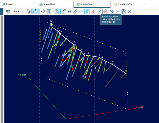
The first way is to select collars individually in the scene:
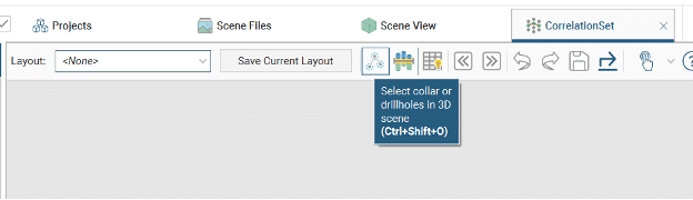
The second way is slicing the scene and clicking “Select all visible collars” (Ctrl+A):
This drillhole set will allow you to see the drillholes you have selected in a 2D view. Drag the drillhole columns of interest into the Correlation Set tab to see them, which you can view as downhole point data with interval data side-by-side to aid your correlation.
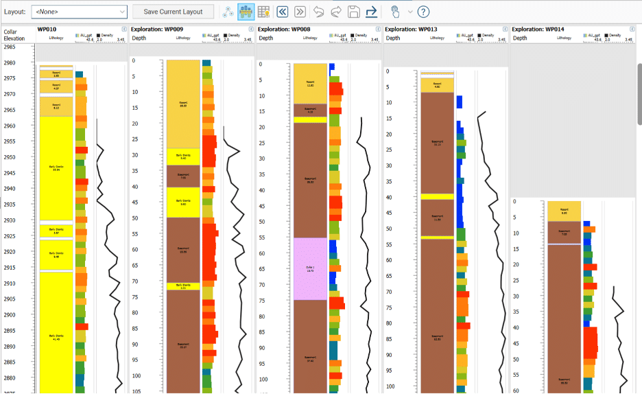
The drillhole correlation tool also allows you to view and work with your data in several different ways. For example, drillholes can be viewed in relative collar elevations, which can be toggled on and off in the toolbar.
The formatting of the Header title information can also be customised to your needs, or category thickness labels can be displayed for lithological or other category data. If working with numeric data, you can also add custom colourmaps and labels and the data can be log transformed.
This tool also makes it possible to customise your column width to maximise screen usage inside the correlation tab. Individual drillholes can be collapsed, or all drillholes can be expanded and collapsed, allowing you to track progress while working and ensure you’re looking at the specific data required.
Finally, a depth filter is available and the ‘apply to all’ setting increases usability which means that drilling data can be plotted as true vertical depth as well as downhole depth. If desired, the depth axis intervals can be more specifically edited to improve snapping behaviour.
Pretty neat, huh?
#2 Need to thin down big data tables? Use the Modulo (%) operation
Did you know the % symbol has two functions in Leapfrog Geo? The first is quite well known. You can use the % symbol as the wildcard value in the Query Filter.
For example, HoleID LIKE EX19% will return any hole names that begin with EX19 and are followed by any other character.
A function that is less commonly known is the % symbol serving as an arithmetic “Modulo” operation. A Modulo operation finds the remainder after dividing one value by another (sometimes called the “modulus”).
Let’s take two non-zero or non-negative values: A (the dividend) and B (the divisor). The remainder of A/B is known as N, the Modulo (also referred to as ‘Mod N’). This operation will therefore produce the remainder, rather than the actual integer quotient.
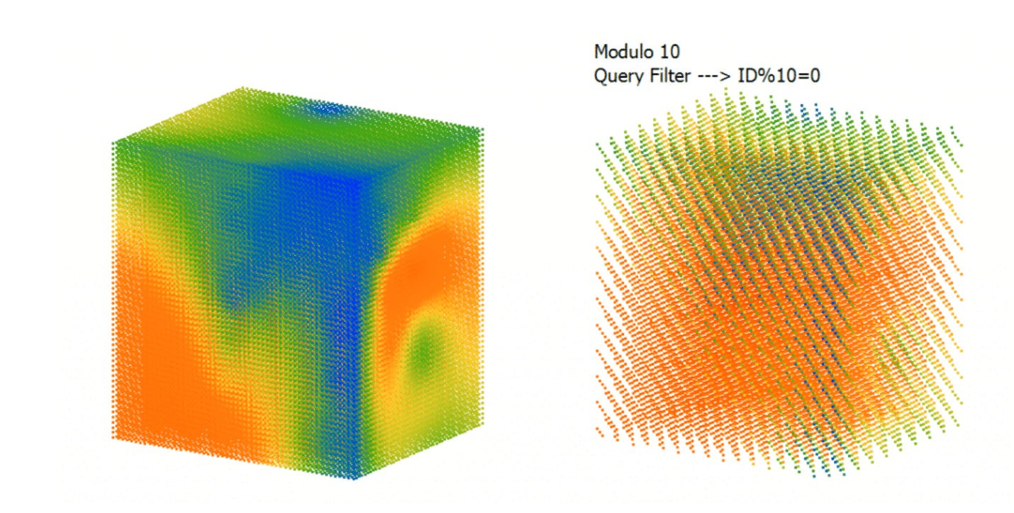
This Modulo operation is particularly handy when trying to thin out large datasets. For example, say you only want to keep every 5th, 10th, or even 50th point.
Using the modulo operation ID%5=0, a Leapfrog query filter will select out only every 5th value. Each row in an object’s table has a unique ID and this operation divides each row ID by the designated value (“5” in this example) and will keep values with a remainder of 0.
Note: Don’t be tempted to use this query for topography! We recommend using the Error Threshold in Triangulated Meshes to simplify large topographic data sets by removing points that do not significantly contribute to the shape of the surface.
This should allow you to get a completely different, and usually useful, insight into your modelled data.
#3 Want to take your surface editing to the next level? Try boundary filters
Turning the Boundary filter off allows Leapfrog to use data outside of the model boundary or fault boundary into order to influence the surface. If a surface is not doing what you expect it to do, remember the Boundary filter is on by default and that turning it off may help.
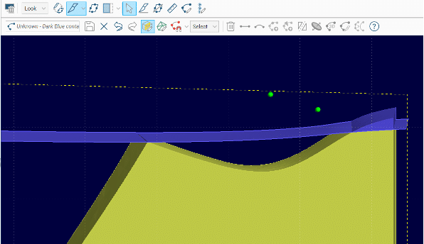
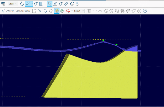
In the image below, the dark blue surface is not honouring the editing points that were added to remove an unwanted sliver of blue unit appearing along the fault.
These editing points are not being honoured, because the Topography is being used as the upper boundary of the model, and, by default, the model will filter out input beyond this boundary.
This means that the points that were added cannot influence the blue surface of the geological model until the Boundary filter is turned off.
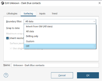
Double-click on the surface of interest in the Project Tree, navigate to the Surfacing tab, and then select “Off” in the Boundary filter dropdown.
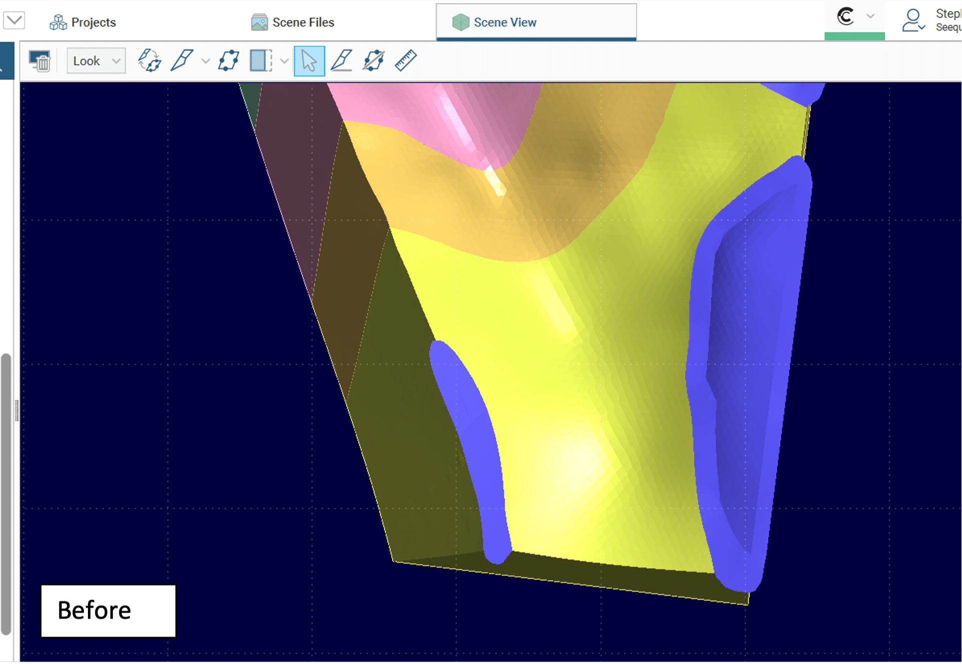
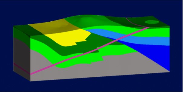
Once this has been done, Leapfrog uses data points outside of the model (or fault block) boundary to influence the geological model, as seen below in the Before and After:
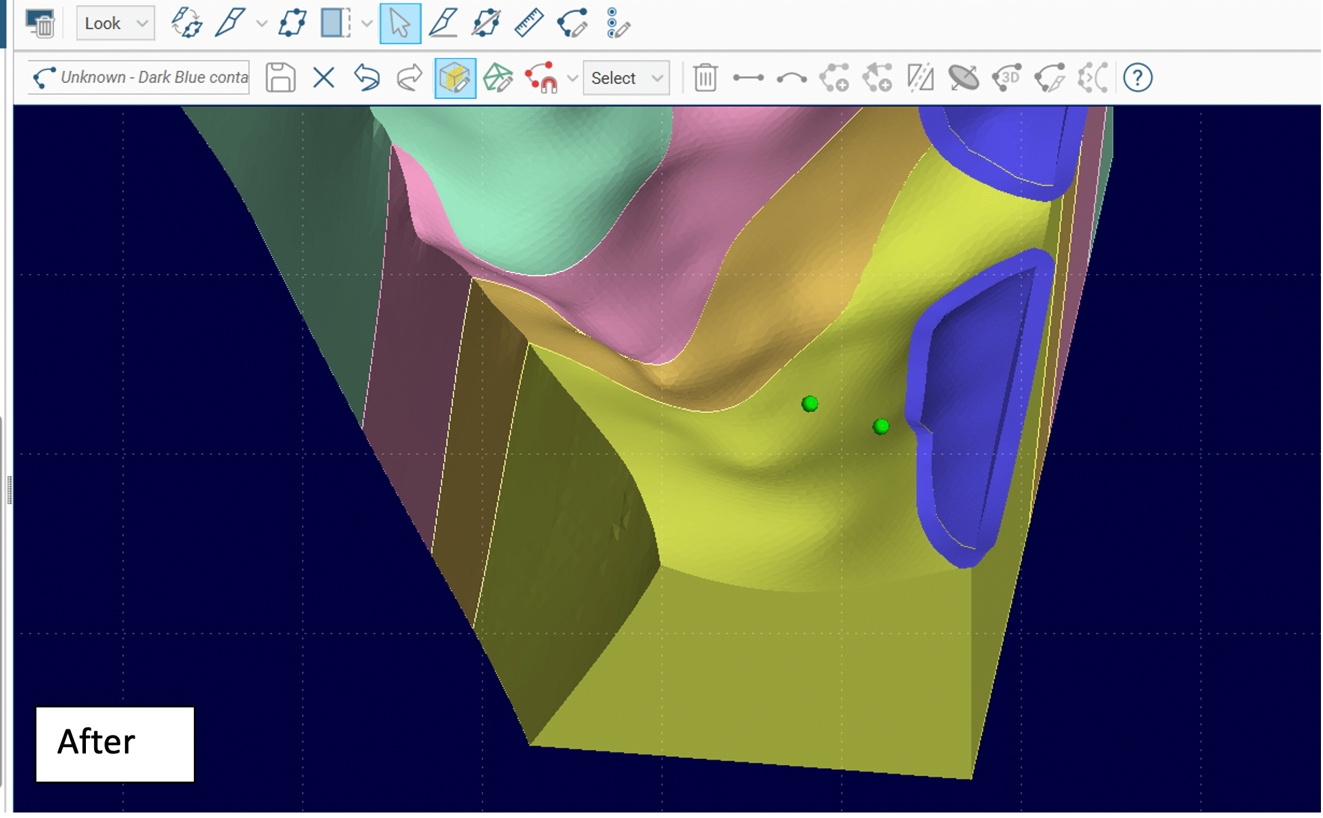
Here is what the original slicer perspective looks like after the Boundary filter has been turned off:
This is also particularly useful for controlling which units are faulted between fault blocks. If you have a set of dykes which were emplaced post-faulting, you can turn the boundary filter off specifically for these dyke units, and your dykes will appear un-faulted and continuous through your fault block boundaries.
Pull in the boundary and all the inputs for the problematic surface to the scene and see if the data is inside of the boundary.
If data exists outside of the boundary, then it might be necessary to turn the Boundary Filter off or customize Boundary filter settings for specific inputs to a surface.
#4 Looking to categorise your polylines? Use the new Polyline attribute feature
One of the standout features in Leapfrog 2024.1 is Polyline Attribution, offering new ways to model your projects by categorising polyline paths as text, numeric, date, or timestamp attributes.
Bring in polylines and their attributes as CSVs. Attributes will upload with your naming conventions intact.
View your attributes under the polyline object in the project tree and display them in your scene.
Write query filters to filter your attributes by name, date, lithology, or alteration. Apply these query filters to display specific attributes, like lithology codes, for quick insights or incorporation into your surfaces.
This feature speeds up mapping data integration, enhances the visualisation of line-based information, and unlocks the value of attributed data—streamlining your mapping, modelling, and classification workflows.

We hope these tips and tricks help you get the most of out of Leapfrog Geo and speed up your workflows so that you can spend less time working with data and more time interpreting geology.