Numerical Modelling best practices in Leapfrog Geo

We will take a deeper look at how Leapfrog Geo constructs a numerical model in order to build upon and provide a better understanding of the tools available at your disposal.

Video Transcript

1
00:00:11,105 –> 00:00:14,420
<v Suzzana>All right, hello and welcome everyone.</v>

2
00:00:14,420 –> 00:00:16,324
I make that 10 o’clock here in the UK.

3
00:00:16,324 –> 00:00:19,231
And so, let’s get started.

4
00:00:19,231 –> 00:00:23,050
Thank you for joining us today for this tech talk

5
00:00:23,050 –> 00:00:26,373
on Numeric Modelling in Leapfrog Geo.

6
00:00:26,373 –> 00:00:29,290
By way of introduction, my name is Suzanna.

7
00:00:29,290 –> 00:00:33,624
I’m a Geologist by background, based out of our UK office.

8
00:00:33,624 –> 00:00:36,510
With me today are my colleagues,

9
00:00:36,510 –> 00:00:39,930
James and Andre, both of whom will be on hand to help

10
00:00:39,930 –> 00:00:41,658
run this session.

11
00:00:41,658 –> 00:00:44,680
Now, our aim for this session is

12
00:00:44,680 –> 00:00:48,204
to really focus in on the interpolant settings

13
00:00:48,204 –> 00:00:52,240
that will most effectively improve your numeric models

14
00:00:52,240 –> 00:00:54,320
from the word go.

15
00:00:54,320 –> 00:00:56,820
Let me set the scene for my project today.

16
00:00:56,820 –> 00:00:59,817
This is a copper gold porphyry deposit.

17
00:00:59,817 –> 00:01:01,325
And from the stats,

18
00:01:01,325 –> 00:01:06,325
we know that it is our Early Diorite unit

19
00:01:06,920 –> 00:01:10,560
that is our highest grade domain.

20
00:01:10,560 –> 00:01:13,220
For the purpose of today’s session,

21
00:01:13,220 –> 00:01:17,081
I’m going to focus on modelling the gold assay information,

22
00:01:17,081 –> 00:01:20,650
so from these drillholes, but in reality,

23
00:01:20,650 –> 00:01:24,750
I could choose to model any type of numerical value here,

24
00:01:26,320 –> 00:01:29,010
for example, RQD data.

25
00:01:29,010 –> 00:01:31,160
If that is the workflow that you’re interested in,

26
00:01:31,160 –> 00:01:34,197
then I’d recommend you head over to the Seequent website,

27
00:01:34,197 –> 00:01:36,560
where there are a couple of videos

28
00:01:36,560 –> 00:01:38,713
on this topic already available.

29
00:01:40,000 –> 00:01:44,520
So coming down to my Numeric Models folder,

30
00:01:44,520 –> 00:01:48,730
I’m now going to select a new RBF interpolant.

31
00:01:51,500 –> 00:01:53,840
And in the first window,

32
00:01:53,840 –> 00:01:58,103
start to specify my initial inputs and outputs.

33
00:01:59,310 –> 00:02:02,130
First, I’m going to want to specify

34
00:02:02,130 –> 00:02:04,440
some suitable numeric values.

35
00:02:04,440 –> 00:02:05,720
So in this case,

36
00:02:05,720 –> 00:02:09,463
I’m going to use my composited gold assay table,

37
00:02:10,407 –> 00:02:15,407
but I can also choose to apply any applicable query filter.

38
00:02:15,800 –> 00:02:20,658
Now, in this case, as part of my initial validation steps,

39
00:02:20,658 –> 00:02:25,658
I actually created a new column in my collar table

40
00:02:25,847 –> 00:02:30,847
called ‘Valid’ simply to help me identify which drillholes

41
00:02:32,300 –> 00:02:35,017
I want to use in my modelling.

42
00:02:35,017 –> 00:02:37,380
I did this by first of all,

43
00:02:37,380 –> 00:02:40,640
creating a new category selection

44
00:02:40,640 –> 00:02:42,430
to make those initial selections

45
00:02:43,320 –> 00:02:46,776
then created a very simple query filter

46
00:02:46,776 –> 00:02:51,776
simply to exclude any of those that are invalid.

47
00:02:51,900 –> 00:02:53,830
And actually for the most part,

48
00:02:53,830 –> 00:02:57,290
it’s just this one hole at the bottom

49
00:02:57,290 –> 00:02:58,963
that I chose to exclude.

50
00:03:00,960 –> 00:03:04,416
As I work on my interpretation or indeed bring in more data,

51
00:03:04,416 –> 00:03:07,000
then it’s always useful to have flexibility

52
00:03:07,000 –> 00:03:10,310
like this built into your drillhole management workflow.

53
00:03:10,310 –> 00:03:13,580
So I would encourage you to set up something similar

54
00:03:13,580 –> 00:03:15,243
if not already done so.

55
00:03:16,189 –> 00:03:20,660
But for now though, let me just go back to my

56
00:03:20,660 –> 00:03:23,973
RBF interpolant definition again,

57
00:03:25,791 –> 00:03:30,791
and let’s start to talk about the interpolant boundary.

58
00:03:32,950 –> 00:03:37,950
Now, the default here is set to be our clipping boundary.

59
00:03:40,850 –> 00:03:42,660
If you don’t know what that is,

60
00:03:42,660 –> 00:03:43,700
or if you want to set that,

61
00:03:43,700 –> 00:03:46,130
then you can actually do that from either the Topography

62
00:03:46,130 –> 00:03:49,950
or indeed the GIS data folder.

63
00:03:49,950 –> 00:03:54,360
So I could choose to manually change this boundary

64
00:03:54,360 –> 00:03:58,360
or to enclose it around any object

65
00:03:58,360 –> 00:03:59,920
that already exists in my project,

66
00:03:59,920 –> 00:04:04,663
or indeed an existing model boundary or volume.

67
00:04:05,960 –> 00:04:09,950
Whatever I set here in my interpolant boundary

68
00:04:09,950 –> 00:04:13,788
is going to be linked to the surface filter,

69
00:04:13,788 –> 00:04:17,350
or by default, is linked to the surface filter

70
00:04:17,350 –> 00:04:22,023
which in itself controls which values can go into the model.

71
00:04:22,920 –> 00:04:27,220
I’m just going to bring a quick slice view into my scene,

72
00:04:27,220 –> 00:04:28,955
just to sort of help us visualise

73
00:04:28,955 –> 00:04:31,183
what I’m about to talk about.

74
00:04:32,020 –> 00:04:33,180
But I will explain this, as this is

75
00:04:33,180 –> 00:04:36,531
basically just a slice of my geological model

76
00:04:36,531 –> 00:04:41,423
just with those sort of gold values seen in the scene here.

77
00:04:43,120 –> 00:04:45,960
Typically your interpolant boundary

78
00:04:45,960 –> 00:04:50,170
would be set to enclose the entire data set.

79
00:04:51,490 –> 00:04:56,150
In which case, all of your specified input values

80
00:04:56,150 –> 00:04:57,570
will become interpolated.

81
00:04:57,570 –> 00:05:00,150
So that’s kind of what we’re seeing in the scene at the moment.

82
00:05:00,150 –> 00:05:02,975
It’s just a simple view of everything

83
00:05:02,975 –> 00:05:06,833
that’s in my data and in my project.

84
00:05:08,380 –> 00:05:09,746
I could choose however,

85
00:05:09,746 –> 00:05:14,380
to set a boundary around an existing volume.

86
00:05:14,380 –> 00:05:15,320
So for example,

87
00:05:15,320 –> 00:05:18,320
if I want to just specifically look at my Early Diorite

88
00:05:18,320 –> 00:05:19,963
which is anything here in green,

89
00:05:20,830 –> 00:05:23,550
then I can choose to do that.

90
00:05:23,550 –> 00:05:28,550
And if I just turn that on now, then you can see,

91
00:05:28,950 –> 00:05:32,090
we’re just seeing that limited subset

92
00:05:32,090 –> 00:05:34,303
of input values in that case.

93
00:05:35,187 –> 00:05:39,230
Now, interestingly, if I wanted to at this point

94
00:05:39,230 –> 00:05:42,900
mimic a soft boundary around the Early Diorite,

95
00:05:42,900 –> 00:05:47,180
So for example, some sort of value buffer

96
00:05:47,180 –> 00:05:49,853
say it’s about 50 meters away,

97
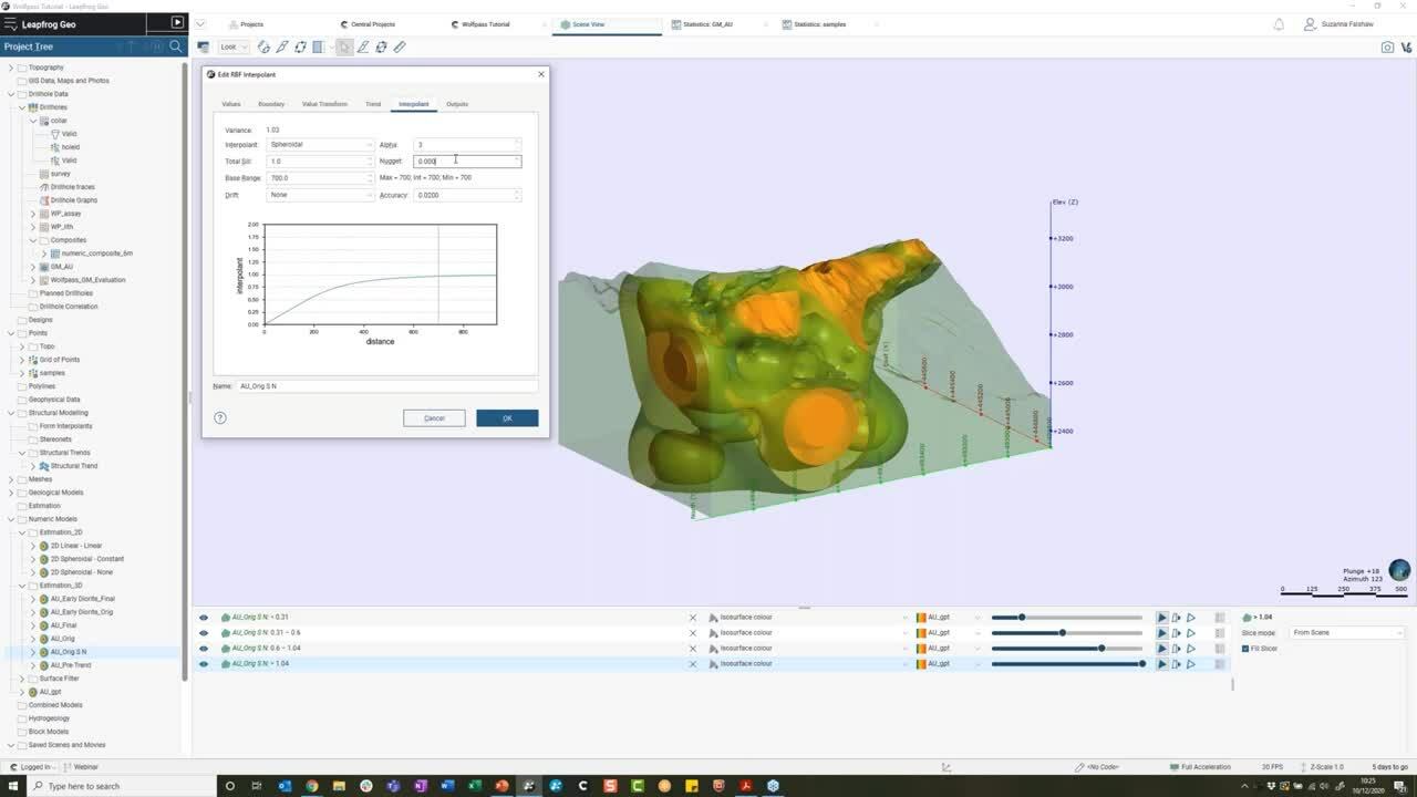
00:05:50,800 –> 00:05:52,723
which is this orange line here.

98
00:05:53,700 –> 00:05:58,683
Then I could incorporate this also into my Surface Filter.

99
00:06:00,300 –> 00:06:02,240
And again, by doing, say,

100
00:06:02,240 –> 00:06:07,240
so if I now select this distance function here,

101
00:06:08,260 –> 00:06:12,270
then again, we’re going to see this update

102
00:06:12,270 –> 00:06:16,393
on which input values can be used into the model.

103
00:06:17,610 –> 00:06:20,610
But now though let’s not complicate things too much.

104
00:06:20,610 –> 00:06:24,480
I’m just simply going to use the same boundary

105
00:06:25,330 –> 00:06:27,803
as my geological model.

106
00:06:28,870 –> 00:06:33,196
And I’m also going to bring down my surface resolution

107
00:06:33,196 –> 00:06:35,630
to something a bit more reasonable.

108
00:06:35,630 –> 00:06:39,580
Now, a rule of thumb with drillhole data would be

109
00:06:39,580 –> 00:06:42,690
to set this to your composite length.

110
00:06:42,690 –> 00:06:45,752
So as to equal the triangulation

111
00:06:45,752 –> 00:06:48,980
or indeed some multiple of this,

112
00:06:48,980 –> 00:06:52,752
if you find the processing time takes too much of a hit.

113
00:06:52,752 –> 00:06:55,360
For this particular data set,

114
00:06:55,360 –> 00:06:59,169
I have six metre length composites already defined.

115
00:06:59,169 –> 00:07:02,800
So I’m going to bring surface resolution down

116
00:07:02,800 –> 00:07:04,913
to multiple of that, 12 in this case.

117
00:07:06,490 –> 00:07:08,660
And of course those composites are there

118
00:07:08,660 –> 00:07:10,400
in order to help normalise

119
00:07:10,400 –> 00:07:12,913
and reduce the variance of my data.

120
00:07:13,870 –> 00:07:18,770
If I didn’t already have numeric composites set up

121
00:07:18,770 –> 00:07:21,186
in my Drillhole Data folder,

122
00:07:21,186 –> 00:07:25,770
then I could actually go into find these here

123
00:07:25,770 –> 00:07:27,193
as well directly.

124
00:07:28,608 –> 00:07:31,840
But now though, let me just go back and use those,

125
00:07:31,840 –> 00:07:33,483
those composites that I have,

126
00:07:35,180 –> 00:07:39,133
and for now, let’s just say OK to this and let it run.

127
00:07:44,920 –> 00:07:47,884
All right, now, there will be some times here

128
00:07:47,884 –> 00:07:51,179
that it’s going to be easier just to jump into models

129
00:07:51,179 –> 00:07:52,817
that have already been set up

130
00:07:52,817 –> 00:07:54,940
and I think this is one of those cases.

131
00:07:54,940 –> 00:07:59,723
So let me just bring in what that is going to generate,

132
00:08:02,120 –> 00:08:07,120
which is essentially our first pass gold numeric model.

133
00:08:09,980 –> 00:08:12,330
If I stick the legend on,

134
00:08:12,330 –> 00:08:14,030
then you’ll start to get idea

135
00:08:14,030 –> 00:08:16,163
or a reference point for that grade.

136
00:08:17,390 –> 00:08:21,680
Now, the power of Leapfrog’s RBF engine

137
00:08:21,680 –> 00:08:25,780
is in its ability to estimate a quantity

138
00:08:25,780 –> 00:08:29,760
into an unknown point by using known drillhole

139
00:08:29,760 –> 00:08:31,830
or point data.

140
00:08:31,830 –> 00:08:33,540
It’s important however,

141
00:08:33,540 –> 00:08:36,770
that when we estimate those unknown points

142
00:08:36,770 –> 00:08:40,383
that we’re selecting an interpolation function,

143
00:08:40,383 –> 00:08:43,570
that will make the most geological sense.

144
00:08:44,730 –> 00:08:47,220
At this first pass stage,

145
00:08:47,220 –> 00:08:49,732
I hope you’ll agree that we’re seeing something

146
00:08:49,732 –> 00:08:52,110
that’s very unrealistic,

147
00:08:52,110 –> 00:08:56,520
especially in regards to this higher grade sort of blow outs

148
00:08:56,520 –> 00:08:58,263
in my Northwest corner.

149
00:09:00,680 –> 00:09:03,970
It’s fairly common for our projects

150
00:09:03,970 –> 00:09:07,320
to have some areas of data scarcity.

151
00:09:07,320 –> 00:09:09,910
If I bring my drillholes in here,

152
00:09:11,086 –> 00:09:13,393
and just turn the filter off for a second,

153
00:09:17,330 –> 00:09:21,639
then I’m sure you agree that sometimes at depth

154
00:09:21,639 –> 00:09:25,280
or indeed on our last full extents,

155
00:09:25,280 –> 00:09:29,060
that we might just not have any drilling information

156
00:09:29,060 –> 00:09:30,103
in that area.

157
00:09:31,740 –> 00:09:32,960
And in this case,

158
00:09:32,960 –> 00:09:36,852
it is the, it’s just three drillholes here.

159
00:09:36,852 –> 00:09:40,493
If I put my filter on,

160
00:09:42,370 –> 00:09:45,241
you can see that it’s just these three drillholes

161
00:09:45,241 –> 00:09:49,640
that are simply causing that interpolation, here,

162
00:09:49,640 –> 00:09:53,340
to become really quite extrapolated.

163
00:09:53,340 –> 00:09:56,620
And unfortunately there’s many an extreme example in line

164
00:09:56,620 –> 00:09:57,660
of such models

165
00:09:57,660 –> 00:10:01,333
as these finding their way into company reporting.

166
00:10:02,220 –> 00:10:04,890
So what I would encourage you all to do,

167
00:10:04,890 –> 00:10:07,890
is to of course start refining the internal structure

168
00:10:07,890 –> 00:10:11,290
of my model and the majority of the functionality

169
00:10:11,290 –> 00:10:16,290
to do so actually sits under the Interpolant tab.

170
00:10:16,590 –> 00:10:17,640
So if I go to the model

171
00:10:17,640 –> 00:10:20,403
and I’ll go to the one that’s run originally.

172
00:10:22,520 –> 00:10:24,260
So just double-click into it

173
00:10:24,260 –> 00:10:27,133
and I’m going to come to the Interpolant tab.

174
00:10:29,150 –> 00:10:34,150
For now, I’m simply going to change my Interpolant type

175
00:10:34,640 –> 00:10:39,640
to a Spheroidal and change my Drift function to None.

176
00:10:41,240 –> 00:10:43,720
I will come back to this in more detail, but for now,

177
00:10:43,720 –> 00:10:47,380
let me just let that run and we’ll have a look

178
00:10:47,380 –> 00:10:49,553
at what that produces instead.

179
00:10:50,960 –> 00:10:52,220
And again, great,

180
00:10:52,220 –> 00:10:53,803
here’s one I prepared earlier,

181
00:10:58,550 –> 00:11:00,910
which we can now see,

182
00:11:00,910 –> 00:11:02,800
and hopefully you can already see

183
00:11:02,800 –> 00:11:05,630
this big notable difference already,

184
00:11:05,630 –> 00:11:09,060
especially where a high grade

185
00:11:10,130 –> 00:11:13,533
or where that original high-grade was blown out.

186
00:11:15,180 –> 00:11:18,363
This time, if I bring my drillholes back in again,

187
00:11:21,870 –> 00:11:25,677
we can see that high grade interpolation

188
00:11:25,677 –> 00:11:29,310
around those three drillhole still exists,

189
00:11:29,310 –> 00:11:33,013
but just with a much smaller range of influence.

190
00:11:34,040 –> 00:11:38,250
But why is that the case? To help answer that question,

191
00:11:38,250 –> 00:11:42,030
I’m going to try and replicate these RBF and parameters

192
00:11:42,030 –> 00:11:45,290
on a simple 2D grid of points

193
00:11:45,290 –> 00:11:49,850
and this should quite literally help connect the dots

194
00:11:49,850 –> 00:11:52,020
in our 3D picture.

195
00:11:52,020 –> 00:11:54,410
So let me move away from this for a second

196
00:11:54,410 –> 00:11:58,020
and just bring in my grid of points

197
00:11:59,070 –> 00:12:02,760
and a couple of arbitrary samples.

198
00:12:02,760 –> 00:12:07,443
Hopefully you can see those values starting to come through.

199
00:12:11,340 –> 00:12:12,173
Here we go.

200
00:12:14,520 –> 00:12:17,820
So what I’ve done so far for this is,

201
00:12:17,820 –> 00:12:22,820
I have created three new RBF models

202
00:12:24,040 –> 00:12:28,173
in order to estimate these six points shown on screen here.

203
00:12:29,140 –> 00:12:34,140
And then I will come back into each of the Interpolant tabs

204
00:12:34,728 –> 00:12:39,728
in order to adjust the Interpolant and Drift settings.

205
00:12:41,600 –> 00:12:45,243
And that’s just what the naming refers to here.

206
00:12:47,380 –> 00:12:52,380
Now, Leapfrog uses two main interpolant functions,

207
00:12:52,670 –> 00:12:57,530
which in very simple terms will produce different estimates

208
00:12:57,530 –> 00:12:59,190
depending on whether the distance

209
00:12:59,190 –> 00:13:01,308
from our known sample points,

210
00:13:01,308 –> 00:13:05,063
i.e. the range, is taken into consideration.

211
00:13:06,019 –> 00:13:10,360
A linear interpolant will simply assume

212
00:13:10,360 –> 00:13:13,840
that any known values closer to the points

213
00:13:13,840 –> 00:13:15,550
you wish to estimate

214
00:13:15,550 –> 00:13:18,610
we’ll have a proportionally greater influence

215
00:13:18,610 –> 00:13:20,673
than any of those further away.

216
00:13:22,040 –> 00:13:25,480
A spheroidal interpolant on the other hand

217
00:13:25,480 –> 00:13:30,160
assumes that there is a finite range or limit

218
00:13:30,160 –> 00:13:32,700
to the influence of our known data

219
00:13:32,700 –> 00:13:36,141
beyond which this should fall to zero.

220
00:13:36,141 –> 00:13:39,130
You may recognize the resemblance here

221
00:13:39,130 –> 00:13:42,060
to a spherical variogram,

222
00:13:42,060 –> 00:13:45,960
and for the vast majority of metallic ore deposits,

223
00:13:45,960 –> 00:13:49,430
this interpolation type is more applicable.

224
00:13:49,430 –> 00:13:53,240
Exceptions to this, maybe any laterally extensive deposit

225
00:13:53,240 –> 00:13:56,503
like coal or banded iron formations.

226
00:13:57,670 –> 00:14:00,870
So in addition to considering the interpolation method,

227
00:14:00,870 –> 00:14:05,510
we must always also decide how best to control

228
00:14:05,510 –> 00:14:09,308
our estimation in the absence of any data.

229
00:14:09,308 –> 00:14:10,680
In other words,

230
00:14:10,680 –> 00:14:13,510
how should our estimation behave

231
00:14:13,510 –> 00:14:17,490
when we’re past the range of our samples?

232
00:14:17,490 –> 00:14:20,540
Say in the scenario we saw just a minute ago

233
00:14:20,540 –> 00:14:22,483
with those three drillholes.

234
00:14:23,610 –> 00:14:27,140
For this, we need to start defining an appropriate Drift

235
00:14:27,140 –> 00:14:29,240
from the options available.

236
00:14:29,240 –> 00:14:33,300
And I think that was the point that I sort of got into

237
00:14:33,300 –> 00:14:35,340
looking at on my grid.

238
00:14:35,340 –> 00:14:40,340
So at the moment I have a Linear interpolant type

239
00:14:40,670 –> 00:14:42,440
with a Linear Drift shown

240
00:14:43,520 –> 00:14:46,890
and much kind of like the continuous coloured legend

241
00:14:46,890 –> 00:14:48,470
that I have up here,

242
00:14:48,470 –> 00:14:49,560
we’re seeing a linear,

243
00:14:49,560 –> 00:14:52,363
a steady linear trend in our estimation.

244
00:14:54,130 –> 00:14:57,660
The issue is, whilst the estimation around

245
00:14:57,660 –> 00:15:00,497
our known data points is as expected,

246
00:15:00,497 –> 00:15:03,690
the Linear Drift will enable values

247
00:15:03,690 –> 00:15:08,420
to both increase past the highest grade,

248
00:15:08,420 –> 00:15:09,253
so in this case,

249
00:15:09,253 –> 00:15:12,803
we’re sort of upwards to about a grade of 13 here,

250
00:15:13,937 –> 00:15:18,937
as well as go into the negatives past the lowest grade.

251
00:15:21,700 –> 00:15:25,260
So for grade data of this nature,

252
00:15:25,260 –> 00:15:29,010
we’re going to want to reign that estimation in

253
00:15:29,010 –> 00:15:32,653
and start to factor in a range of influence.

254
00:15:34,190 –> 00:15:37,931
So looking now at our spheroidal interpolant

255
00:15:37,931 –> 00:15:41,130
with a Drift of None,

256
00:15:41,130 –> 00:15:44,430
we can see how the range starts to have an influence

257
00:15:44,430 –> 00:15:48,820
on our estimation and then when we move away

258
00:15:48,820 –> 00:15:50,780
from our known values,

259
00:15:50,780 –> 00:15:52,770
so for example, if I start to come out

260
00:15:52,770 –> 00:15:57,770
onto the extents here, then the estimation is falling

261
00:15:57,910 –> 00:16:00,790
or decaying back to zero.

262
00:16:00,790 –> 00:16:02,180
And that will be the same

263
00:16:02,180 –> 00:16:05,000
if I sort of go around any of these,

264
00:16:05,000 –> 00:16:09,338
we would expect to be getting down to a value of zero

265
00:16:09,338 –> 00:16:11,953
away from any data points.

266
00:16:13,760 –> 00:16:16,170
And of course, if you are close to the data point,

267
00:16:16,170 –> 00:16:20,173
we would expect it to be an estimation similar.

268
00:16:21,700 –> 00:16:26,290
So where you’re modelling an unconstrained area,

269
00:16:26,290 –> 00:16:29,770
or perhaps don’t have many low grade holes

270
00:16:29,770 –> 00:16:31,811
to constrain your deposit,

271
00:16:31,811 –> 00:16:34,890
using a Drift of None will ensure

272
00:16:34,890 –> 00:16:38,630
that you have some control on how far your samples

273
00:16:38,630 –> 00:16:40,410
would have an influence.

274
00:16:40,410 –> 00:16:44,500
That said, if you are trying to model something constrained,

275
00:16:44,500 –> 00:16:49,450
for example, the Early Diorite domain that we saw earlier,

276
00:16:49,450 –> 00:16:53,580
then using a Drift function of Constant

277
00:16:54,850 –> 00:16:56,588
could be more applicable.

278
00:16:56,588 –> 00:17:00,480
In this case, our values are reverting

279
00:17:00,480 –> 00:17:03,030
to the approximate mean of the data.

280
00:17:03,030 –> 00:17:08,030
So if I just bring up the statistics, our mean here is 4.167,

281
00:17:12,010 –> 00:17:14,910
which means that as I’m getting to the outskirts,

282
00:17:14,910 –> 00:17:18,960
I would expect it to be coming back towards that mean.

283
00:17:18,960 –> 00:17:22,440
So a few different options, but of course,

284
00:17:22,440 –> 00:17:26,240
different scenarios in how we want to apply these.

285
00:17:26,240 –> 00:17:31,240
Now, if I jump back now to my gold model,

286
00:17:35,070 –> 00:17:36,580
then let’s start first of all,

287
00:17:36,580 –> 00:17:39,513
just with a quick reminder of where we started.

288
00:17:41,280 –> 00:17:43,003
Which was with this model,

289
00:17:44,170 –> 00:17:48,650
and this is applying that default Linear interpolant,

290
00:17:49,530 –> 00:17:54,030
and that simply by changing this already

291
00:17:54,030 –> 00:17:58,360
to the spheroidal interpolant type

292
00:17:58,360 –> 00:18:00,593
along with a Drift of None,

293
00:18:02,010 –> 00:18:04,330
then we’re starting to see something

294
00:18:04,330 –> 00:18:06,653
that makes much more sense.

295
00:18:08,791 –> 00:18:13,791
So if I go back now and go back to my Interpolant tab

296
00:18:15,870 –> 00:18:18,473
to sort of look at some of these other settings.

297
00:18:20,924 –> 00:18:25,924
So far we know we want to limit the influence

298
00:18:27,030 –> 00:18:30,820
of our known data to a certain distance,

299
00:18:30,820 –> 00:18:33,020
and that it’s the distance reign

300
00:18:33,020 –> 00:18:36,243
essentially controlling that correlation.

301
00:18:37,230 –> 00:18:40,110
It’s reasonable, therefore that you’re going to want to,

302
00:18:40,110 –> 00:18:42,610
you’re going to want to change the Base Range

303
00:18:42,610 –> 00:18:44,720
to something more appropriate.

304
00:18:44,720 –> 00:18:46,170
And if you don’t know where to start,

305
00:18:46,170 –> 00:18:49,680
then a rule of thumb could be around twice

306
00:18:49,680 –> 00:18:51,240
the drillhole spacing.

307
00:18:51,240 –> 00:18:55,170
So in this case, let’s up that to around 700,

308
00:18:55,170 –> 00:18:57,393
which is appropriate for this project.

309
00:18:59,350 –> 00:19:04,000
We also want to consider our Nugget and in Leapfrog,

310
00:19:04,000 –> 00:19:07,813
this is expressed as a percentage to our sill.

311
00:19:09,070 –> 00:19:13,640
Increasing the value of the Nugget will create smoother

312
00:19:13,640 –> 00:19:18,640
results by limiting the effects of extreme outliers.

313
00:19:18,660 –> 00:19:21,972
In other words, we would give more emphasis

314
00:19:21,972 –> 00:19:26,190
to the average grades of our surrounding values

315
00:19:26,190 –> 00:19:28,643
and less on the actual data point.

316
00:19:29,490 –> 00:19:32,330
It can basically help to reduce noise

317
00:19:32,330 –> 00:19:34,630
caused by these outliers

318
00:19:34,630 –> 00:19:37,703
or with inaccurately measured samples.

319
00:19:39,090 –> 00:19:43,420
What value to use here is very much decided on a deposit

320
00:19:43,420 –> 00:19:44,780
by deposit case.

321
00:19:44,780 –> 00:19:48,500
And by all means, if you or someone else

322
00:19:48,500 –> 00:19:51,060
in your organisation has already figured this out

323
00:19:52,030 –> 00:19:54,703
for your deposit, then by all means apply it here.

324
00:19:55,570 –> 00:19:58,970
Perhaps for a gold deposit like this

325
00:19:58,970 –> 00:20:02,280
then a rule of thumb will be,

326
00:20:02,280 –> 00:20:05,410
let’s say, 20 to 30% of the Sill.

327
00:20:05,410 –> 00:20:07,170
So let’s just take this down.

328
00:20:07,170 –> 00:20:10,793
For example, it’s 0.2, which is going to be 20% of that

329
00:20:10,793 –> 00:20:14,170
sill I have. 10% might be more appropriate

330
00:20:14,170 –> 00:20:17,400
for other metallic deposits or indeed none,

331
00:20:17,400 –> 00:20:21,560
if you have a very consistent data set.

332
00:20:21,560 –> 00:20:23,733
We’ve spoken about Drift already,

333
00:20:25,220 –> 00:20:29,430
but now that we are past the range of influence,

334
00:20:29,430 –> 00:20:33,520
then it’s really our drift that comes into play.

335
00:20:33,520 –> 00:20:37,220
Using None in this case is going to help

336
00:20:37,220 –> 00:20:41,409
control how far my samples will have an influence

337
00:20:41,409 –> 00:20:45,223
before the estimation decays back to zero.

338
00:20:46,329 –> 00:20:50,140
I’m not going to delve too much

339
00:20:50,140 –> 00:20:51,850
into the other settings here.

340
00:20:51,850 –> 00:20:53,410
You can always read about these

341
00:20:53,410 –> 00:20:55,323
to your heart’s content online,

342
00:20:56,250 –> 00:20:58,720
but the take home point really is that,

343
00:20:58,720 –> 00:21:03,320
it’s the interpolant the Base Range,

344
00:21:03,320 –> 00:21:06,940
that percentage Nugget to the sill and Drift

345
00:21:07,840 –> 00:21:10,480
that will have the most material effects

346
00:21:10,480 –> 00:21:13,400
on your numeric model.

347
00:21:13,400 –> 00:21:16,030
Get these right and you should be well on your way

348
00:21:16,030 –> 00:21:17,970
to producing a robust model

349
00:21:17,970 –> 00:21:21,060
that makes the best of your geological knowledge.

350
00:21:21,060 –> 00:21:24,460
All right, now we’ve talked a little bit about

351
00:21:24,460 –> 00:21:27,310
these interpolant settings.

352
00:21:27,310 –> 00:21:30,706
I thought it would be worth a quick run over

353
00:21:30,706 –> 00:21:33,750
on the Isosurfaces.

354
00:21:33,750 –> 00:21:35,860
So we can see all these,

355
00:21:35,860 –> 00:21:39,530
as we expand out our numeric model objects,

356
00:21:39,530 –> 00:21:41,520
we’ve got Isosurfaces

357
00:21:41,520 –> 00:21:45,420
and then of course the resulting Output Volumes.

358
00:21:45,420 –> 00:21:50,020
When we pick cutoffs in our Outputs tab,

359
00:21:50,020 –> 00:21:54,047
we are simply asking Leapfrog to define some boundaries

360
00:21:54,047 –> 00:21:56,990
in space, i.e. contours,

361
00:21:56,990 –> 00:22:00,520
where there is the same consistent grade.

362
00:22:00,520 –> 00:22:05,520
Essentially the Isosurfaces perform the exact same task

363
00:22:05,910 –> 00:22:08,696
as our geological surfaces do

364
00:22:08,696 –> 00:22:10,776
when we’re geologically modeling.

365
00:22:10,776 –> 00:22:14,690
But instead of building these surfaces ourselves,

366
00:22:14,690 –> 00:22:17,051
we’re simply picking grade boundaries

367
00:22:17,051 –> 00:22:20,330
that we want to see and Leapfrog will go

368
00:22:20,330 –> 00:22:21,973
and build them for us.

369
00:22:23,250 –> 00:22:26,343
It is this contour surface that,

370
00:22:26,343 –> 00:22:29,770
that we’re seeing here in 3D.

371
00:22:29,770 –> 00:22:34,020
And if we want to visualise a specific value,

372
00:22:34,020 –> 00:22:38,857
then we can do so by updating the Iso Values here.

373
00:22:40,760 –> 00:22:44,850
Before I do that, let me just jump back

374
00:22:44,850 –> 00:22:46,980
into the grid of points,

375
00:22:46,980 –> 00:22:51,430
just to highlight this on a sort of simpler dataset.

376
00:22:53,947 –> 00:22:58,810
So back in with my grid of points, let’s say for instance,

377
00:22:58,810 –> 00:23:03,350
I now want to visualise a contour surface

378
00:23:03,350 –> 00:23:07,612
with a grade of two, then I can replicate that here

379
00:23:07,612 –> 00:23:12,049
simply by setting some appropriate value filters.

380
00:23:12,049 –> 00:23:14,520
And we can see that now

381
00:23:14,520 –> 00:23:18,746
sort of finding all of those sort of values of two in space.

382
00:23:18,746 –> 00:23:22,840
And these it’s this point that of course

383
00:23:22,840 –> 00:23:25,263
is going to become our contour.

384
00:23:27,900 –> 00:23:29,401
For the hikers amongst us

385
00:23:29,401 –> 00:23:32,550
who are maybe used to seeing elevation contour lines

386
00:23:32,550 –> 00:23:33,850
on a 2D map

387
00:23:33,850 –> 00:23:35,492
this is the same principle,

388
00:23:35,492 –> 00:23:38,180
except in the case of our gold model,

389
00:23:38,180 –> 00:23:41,803
we’re simply looking at a value representation in 3D.

390
00:23:43,060 –> 00:23:48,060
So let me go back to my gold model once again

391
00:23:49,690 –> 00:23:54,690
and actually set some better Iso Values for this deposit.

392
00:23:57,710 –> 00:23:59,960
So am just going to go double-click back in

393
00:23:59,960 –> 00:24:02,870
and head over to the Output tab.

394
00:24:02,870 –> 00:24:06,670
So let’s just set a few, make a little bit more sense

395
00:24:06,670 –> 00:24:10,900
than the ones that are put in as default.

396
00:24:10,900 –> 00:24:14,663
So let’s say 0.5, 0.75,

397
00:24:16,350 –> 00:24:21,350
let’s do a 1, a 1.25 and a 1.5, I think we’ll suffice.

398
00:24:27,970 –> 00:24:29,640
The other thing that I’m going to do

399
00:24:29,640 –> 00:24:33,990
is take down the resolution on my higher grades

400
00:24:33,990 –> 00:24:37,023
to try and be as accurate as possible.

401
00:24:38,190 –> 00:24:41,360
And remembering to know you might not have heard it,

402
00:24:41,360 –> 00:24:43,650
but remembering my much earlier points

403
00:24:43,650 –> 00:24:46,010
about matching this where possible

404
00:24:46,010 –> 00:24:48,500
to the drillhole composite lengths.

405
00:24:48,500 –> 00:24:51,963
So that’s why I’m sort of picking the six here.

406
00:24:53,500 –> 00:24:58,500
There’s also the ability in this tab to clamp output values,

407
00:24:59,740 –> 00:25:02,610
the default assumption is that

408
00:25:02,610 –> 00:25:04,320
nothing should fall below zero,

409
00:25:04,320 –> 00:25:07,151
which is why we’re seeing that clamp,

410
00:25:07,151 –> 00:25:11,440
but you can always change that if need be likewise,

411
00:25:11,440 –> 00:25:13,763
you can set different Lower,

412
00:25:14,710 –> 00:25:19,280
and indeed Upper bounds in the Value Transform tab

413
00:25:19,280 –> 00:25:22,373
to cap any values you may deem too low or too high,

414
00:25:23,360 –> 00:25:26,803
but I’m not going to focus on that for now.

415
00:25:28,110 –> 00:25:31,230
So let me just let that run

416
00:25:37,030 –> 00:25:42,030
and again, in the magic of Leapfrog,

417
00:25:42,510 –> 00:25:46,940
so have a look at, so what that has produced,

418
00:25:46,940 –> 00:25:50,630
and again, we’re starting to see something visually

419
00:25:50,630 –> 00:25:52,710
that perhaps makes more sense.

420
00:25:52,710 –> 00:25:57,033
That makes more sense to us and to our gold boundaries.

421
00:25:58,990 –> 00:26:03,010
Now, if I want to see more connectivity

422
00:26:03,010 –> 00:26:07,550
between my drillholes, then aside from the Base Range,

423
00:26:07,550 –> 00:26:09,630
I could use a trend for this.

424
00:26:09,630 –> 00:26:14,630
Also the central shear zone, for example,

425
00:26:15,720 –> 00:26:20,720
is no doubt playing a dominant structural control

426
00:26:21,870 –> 00:26:23,750
on my mineralisation.

427
00:26:23,750 –> 00:26:25,490
Starting to see a lot of our high grades,

428
00:26:25,490 –> 00:26:28,463
sort of following some sort of trend here.

429
00:26:29,370 –> 00:26:32,400
So applying a structural trend should help

430
00:26:32,400 –> 00:26:36,409
to account for any changes in the strength

431
00:26:36,409 –> 00:26:40,313
and direction of continuity along this ridge.

432
00:26:41,330 –> 00:26:45,373
I’ve already defined a Structural Trend for the shear zone.

433
00:26:46,230 –> 00:26:49,173
I sort of put it as something like this for now.

434
00:26:51,130 –> 00:26:55,410
However we could of course always update this as need be.

435
00:26:55,410 –> 00:26:58,640
Either way, this is a typical step to take

436
00:26:58,640 –> 00:27:02,243
given that nature is very rarely isotropic.

437
00:27:03,530 –> 00:27:08,530
So let me go and apply this Structural Trend to my model

438
00:27:11,960 –> 00:27:15,403
and which I can do from my Trend tab.

439
00:27:17,790 –> 00:27:20,220
And I’ve only got the one in my project at the moment,

440
00:27:20,220 –> 00:27:22,353
So it’s just that Structural Trend,

441
00:27:25,240 –> 00:27:26,793
and let’s just let that run.

442
00:27:34,000 –> 00:27:39,000
And again, in a fantastic here’s one I prepared earlier,

443
00:27:43,430 –> 00:27:45,370
we can see what that has done

444
00:27:45,370 –> 00:27:49,870
this definitely you can see how that trend has changed

445
00:27:49,870 –> 00:27:52,780
there is weighting of points in space

446
00:27:52,780 –> 00:27:57,550
to define that continuity along that ridge.

447
00:27:57,550 –> 00:28:01,560
So though powerful and usually very applicable

448
00:28:01,560 –> 00:28:05,776
certainly in our sort of metallic gold

449
00:28:05,776 –> 00:28:08,653
or indeed any deposit.

450
00:28:09,970 –> 00:28:13,843
So now that we’ve sort of run to this point,

451
00:28:14,870 –> 00:28:17,030
it’s likely at this stage

452
00:28:17,030 –> 00:28:21,590
that we’re going to want to hone in our mineralised domains.

453
00:28:21,590 –> 00:28:26,147
I spoke earlier about the Early Diorite unit

454
00:28:27,780 –> 00:28:31,650
having our – containing our – highest mean gold grade.

455
00:28:31,650 –> 00:28:36,439
So let’s come full circle and create a Numeric model

456
00:28:36,439 –> 00:28:38,793
for just this volume also.

457
00:28:41,430 –> 00:28:46,430
So let me clear the scene and let me cheat

458
00:28:48,370 –> 00:28:51,640
by copying my last model

459
00:28:51,640 –> 00:28:54,760
with all of its parameters into the new one.

460
00:29:05,230 –> 00:29:10,230
And now we can go into that copy of our model

461
00:29:11,880 –> 00:29:16,750
and start to apply reasonable premises here as well.

462
00:29:16,750 –> 00:29:20,060
Now, the first thing we’re going to want to do is of course,

463
00:29:20,060 –> 00:29:21,470
set some boundary at the moment

464
00:29:21,470 –> 00:29:25,900
it’s just the exact same as the last one,

465
00:29:25,900 –> 00:29:30,760
which is the extents of my geological model.

466
00:29:30,760 –> 00:29:34,830
Say, let’s go in and set a New Lateral Extent.

467
00:29:34,830 –> 00:29:37,971
And what I’m going to do is use the volume

468
00:29:37,971 –> 00:29:41,290
for my geological model as that extent.

469
00:29:41,290 –> 00:29:46,290
Say from surface, and then under my geological models,

470
00:29:48,370 –> 00:29:50,200
under the Output Volumes,

471
00:29:50,200 –> 00:29:52,903
I’m going to select that Early Diorite.

472
00:29:57,230 –> 00:29:59,920
Now, whilst that’s running

473
00:29:59,920 –> 00:30:02,960
remember that what that is going to do

474
00:30:02,960 –> 00:30:06,710
is first of all, constrain your model

475
00:30:06,710 –> 00:30:08,340
to that unit of interest.

476
00:30:08,340 –> 00:30:10,043
So this is my Early Diorite.

477
00:30:12,530 –> 00:30:17,530
And it’s also just only going to use the values

478
00:30:22,910 –> 00:30:26,320
that refer to this unit,

479
00:30:26,320 –> 00:30:29,700
what to do with that initial surface filter set up.

480
00:30:29,700 –> 00:30:30,533
We then of course

481
00:30:30,533 –> 00:30:34,120
want to go and review our interpolant settings here

482
00:30:34,120 –> 00:30:35,693
to check that they’re still applicable

483
00:30:35,693 –> 00:30:39,303
now that we’ve constrained our data to one domain.

484
00:30:40,740 –> 00:30:45,740
Let me say, let me go back and double-click into this model.

485
00:30:46,240 –> 00:30:47,788
And let’s just double check once again,

486
00:30:47,788 –> 00:30:51,493
that our interpolant settings make sense.

487
00:30:52,570 –> 00:30:57,410
It’s probably going to be more applicable in this case

488
00:30:58,635 –> 00:31:01,290
that where we have an absence of data,

489
00:31:01,290 –> 00:31:06,213
so again, on the outskirts, on the extents of our model,

490
00:31:08,460 –> 00:31:10,730
that perhaps we’re going to want to revert

491
00:31:10,730 –> 00:31:13,610
to the mean of the grade in the absence

492
00:31:13,610 –> 00:31:15,103
of any other information.

493
00:31:16,110 –> 00:31:19,030
In which case, the best thing that we can do

494
00:31:19,030 –> 00:31:23,890
is simply to update the Drift here to Constant.

495
00:31:23,890 –> 00:31:26,570
Hopefully you remember from that grid of points,

496
00:31:26,570 –> 00:31:31,200
how that is always going to revert to the mean of the data.

497
00:31:31,200 –> 00:31:32,740
I think for now,

498
00:31:32,740 –> 00:31:35,460
I’m just going to leave every other setting the same,

499
00:31:35,460 –> 00:31:37,630
but of course we could come in

500
00:31:37,630 –> 00:31:41,270
and start to change any of these,

501
00:31:41,270 –> 00:31:44,340
if we wish to see things a little bit differently,

502
00:31:44,340 –> 00:31:47,070
but for now, it’s that drift that for me

503
00:31:47,070 –> 00:31:48,570
is the most important.

504
00:31:48,570 –> 00:31:53,147
So again, let me rerun and bring in a final output.

505
00:32:02,240 –> 00:32:06,520
And if I just make these a little less transparent,

506
00:32:06,520 –> 00:32:08,230
you can hopefully see now

507
00:32:08,230 –> 00:32:13,230
that whereas before we had sort of that those waste grades

508
00:32:14,230 –> 00:32:17,260
coming in on this sort of bottom corner,

509
00:32:17,260 –> 00:32:19,500
we’re now reverting

510
00:32:19,500 –> 00:32:23,330
to something similar to the mean and I think in this case,

511
00:32:23,330 –> 00:32:25,630
if I remember rightly the mean is yeah, 1.151.

512
00:32:29,272 –> 00:32:33,130
So we would expect to be kind of up in that sort of darker,

513
00:32:33,130 –> 00:32:34,433
darker yellow colours.

514
00:32:38,020 –> 00:32:39,620
At this point,

515
00:32:39,620 –> 00:32:42,230
I’m going to say that I’m reasonably happy

516
00:32:42,230 –> 00:32:43,793
with the models I have.

517
00:32:44,720 –> 00:32:47,900
I would, of course, want to interrogate these lot further,

518
00:32:47,900 –> 00:32:50,502
maybe make some manual edits

519
00:32:50,502 –> 00:32:53,578
or double check some of the input data,

520
00:32:53,578 –> 00:32:55,490
but for the purpose of this talk,

521
00:32:55,490 –> 00:32:57,910
I hope that this has gone some way

522
00:32:57,910 –> 00:33:01,090
in highlighting which interpolant settings

523
00:33:01,090 –> 00:33:04,984
will most effectively improve your Numeric Models.

524
00:33:04,984 –> 00:33:08,450
I appreciate that this is a very extensive topic

525
00:33:08,450 –> 00:33:10,550
to try and fit into a shorter amount of time.

526
00:33:10,550 –> 00:33:13,223
Please do keep your questions coming in.

527
00:33:14,090 –> 00:33:15,130
In the meantime,

528
00:33:15,130 –> 00:33:19,030
I’m going to hand over to James now,

529
00:33:19,030 –> 00:33:23,550
to run us through the Indicator RBF Interpolant tool.

530
00:33:24,550 –> 00:33:25,730
<v James>Thanks, Suzanna,</v>

531
00:33:25,730 –> 00:33:28,850
bear with me two seconds and I’ll just share my screen.

532
00:33:28,850 –> 00:33:32,350
So a lot of the stuff that Suzanna has run through

533
00:33:32,350 –> 00:33:34,830
in those settings, we’re going to apply now

534
00:33:34,830 –> 00:33:37,620
to the Indicator Numeric Models.

535
00:33:38,520 –> 00:33:41,530
Indicator Numeric Models are a tool

536
00:33:41,530 –> 00:33:46,220
that is often underused or overlooked in preference

537
00:33:46,220 –> 00:33:47,810
to the RBF models,

538
00:33:47,810 –> 00:33:51,480
but Indicator Models can have a really valuable place

539
00:33:51,480 –> 00:33:52,923
in anyone’s workflow.

540
00:33:53,870 –> 00:33:55,910
So I’ve got the same project here,

541
00:33:55,910 –> 00:33:58,050
but this time I’m going to be looking at

542
00:33:58,050 –> 00:34:02,120
some of the copper grades that we have in the project.

543
00:34:02,120 –> 00:34:06,310
If I go into a bit of analysis initially on my data,

544
00:34:06,310 –> 00:34:09,968
I can see that when I look at the statistics for my copper,

545
00:34:09,968 –> 00:34:14,968
there isn’t really a dominant trend to the geology

546
00:34:16,350 –> 00:34:19,879
and where my copper is hosted is more of a disseminated

547
00:34:19,879 –> 00:34:24,480
mineralization that is spread across multiple domains.

548
00:34:24,480 –> 00:34:27,600
If I come in and have a look at the copper itself,

549
00:34:27,600 –> 00:34:29,250
what I want to try and understand

550
00:34:30,170 –> 00:34:34,740
is what it would be a good cutoff to apply

551
00:34:34,740 –> 00:34:37,580
when I’m trying to use my indicator models

552
00:34:37,580 –> 00:34:38,650
and this case here,

553
00:34:38,650 –> 00:34:42,470
I’ve had a look at the histogram of the log,

554
00:34:42,470 –> 00:34:44,380
and there’s many different ways

555
00:34:44,380 –> 00:34:46,954
that you can approach cutoffs.

556
00:34:46,954 –> 00:34:49,440
But in this case, I’m looking for breaks

557
00:34:49,440 –> 00:34:51,640
in the natural distribution of the data.

558
00:34:51,640 –> 00:34:54,600
And for today, I’m going to pick one around this area

559
00:34:54,600 –> 00:34:56,593
where I see this kind of step change

560
00:34:56,593 –> 00:34:58,573
in my grade distribution.

561
00:34:59,410 –> 00:35:00,900
So at this point here,

562
00:35:00,900 –> 00:35:05,900
I can see that I’m somewhere between 0.28 and 0.31% copper.

563
00:35:06,770 –> 00:35:09,950
So for the purpose of the exercise,

564
00:35:09,950 –> 00:35:13,553
we’ll walk through today we’ll use 0.3 as my cutoff.

565
00:35:15,051 –> 00:35:18,210
So once I’ve had a look at my data and I have a better idea

566
00:35:18,210 –> 00:35:19,660
of the kind of cutoffs

567
00:35:19,660 –> 00:35:23,020
I want to use to identify mineralization,

568
00:35:23,020 –> 00:35:25,773
I can come down to my Numeric Models folder,

569
00:35:26,720 –> 00:35:30,710
right-click to create a New Indicator

570
00:35:30,710 –> 00:35:31,910
Interpolant.

571
00:35:34,186 –> 00:35:38,073
The layout to this is very similar to the Numeric Modelling.

572
00:35:39,010 –> 00:35:39,843
Again, you can see,

573
00:35:39,843 –> 00:35:43,050
that I can specify the values I want to use.

574
00:35:43,050 –> 00:35:45,090
I can pick the boundaries I want to apply.

575
00:35:45,090 –> 00:35:48,700
So for now, I’m just going to use the total project

576
00:35:48,700 –> 00:35:49,533
and all my data.

577
00:35:51,420 –> 00:35:53,730
And if I want to apply my query filters,

578
00:35:53,730 –> 00:35:55,080
I can do that here as well.

579
00:35:56,086 –> 00:35:58,670
A couple of other steps I need to do,

580
00:35:58,670 –> 00:36:00,820
because this is an Indicator Interpolant.

581
00:36:00,820 –> 00:36:02,730
I need to apply a cutoff.

582
00:36:02,730 –> 00:36:03,590
So what I’m doing here is

583
00:36:03,590 –> 00:36:05,960
I’m trying to create a single surface

584
00:36:05,960 –> 00:36:10,513
in closing grades above my cutoff of 0.3.

585
00:36:11,840 –> 00:36:13,240
And for the purpose of time,

586
00:36:13,240 –> 00:36:16,490
I’m also going to just composite my data here.

587
00:36:16,490 –> 00:36:18,710
So that it helps to run,

588
00:36:18,710 –> 00:36:22,770
but it also helps to standardise my data.

589
00:36:22,770 –> 00:36:26,400
So I’m going to set my composite length to four

590
00:36:26,400 –> 00:36:29,240
and anywhere where I have residual lengths less than one,

591
00:36:29,240 –> 00:36:31,990
I’m going to distribute those equally back through my data.

592
00:36:33,950 –> 00:36:36,093
I can give it a name to help me identify it.

593
00:36:37,350 –> 00:36:38,500
And we’re going to come back

594
00:36:38,500 –> 00:36:42,603
and talk about the Iso values in a minute.

595
00:36:43,520 –> 00:36:45,338
So for now, I’m going to leave my Iso value

596
00:36:45,338 –> 00:36:49,003
as a default of 0.5, and then I can let that run.

597
00:36:52,460 –> 00:36:55,580
So what Leapfrog does with the indicators

598
00:36:55,580 –> 00:36:58,090
is it will create two volumes.

599
00:36:58,090 –> 00:37:02,150
It creates a volume that is considered inside my cutoff.

600
00:37:02,150 –> 00:37:05,093
So if I expand my model down here,

601
00:37:06,440 –> 00:37:08,800
we’ll see there’s two volumes as the output.

602
00:37:08,800 –> 00:37:11,960
So there’s one that is above my cutoff,

603
00:37:11,960 –> 00:37:12,960
which is this volume.

604
00:37:12,960 –> 00:37:15,890
And one that is below my cutoff,

605
00:37:15,890 –> 00:37:17,290
which is the Outside volume.

606
00:37:19,775 –> 00:37:20,690
Now, at the moment,

607
00:37:20,690 –> 00:37:23,560
those shapes are not particularly realistic.

608
00:37:23,560 –> 00:37:25,330
Again, very similar to what we saw

609
00:37:25,330 –> 00:37:28,720
with Suzanna’s explanation initially

610
00:37:28,720 –> 00:37:30,100
because of the settings I’m using,

611
00:37:30,100 –> 00:37:32,853
I’m getting these blow outs to the extent of my models.

612
00:37:35,020 –> 00:37:36,388
The other thing we can have a quick look at

613
00:37:36,388 –> 00:37:38,940
before we go and change any of the settings

614
00:37:38,940 –> 00:37:42,550
is how Leapfrog manages the data

615
00:37:42,550 –> 00:37:45,050
that we’ve used in this Indicator.

616
00:37:45,050 –> 00:37:46,850
So it’s taken all of my copper values

617
00:37:46,850 –> 00:37:49,340
and I’ve got my data here in my models.

618
00:37:49,340 –> 00:37:50,563
So if I track that on,

619
00:37:54,503 –> 00:37:56,253
just set that up so you can see it.

620
00:37:57,690 –> 00:38:01,310
So initially from my copper values,

621
00:38:01,310 –> 00:38:04,230
Leapfrog will go and flag all of the data

622
00:38:04,230 –> 00:38:07,060
as either being above or below my cutoff.

623
00:38:07,060 –> 00:38:09,270
So here you can see my cutoff.

624
00:38:09,270 –> 00:38:10,670
So everything above or below.

625
00:38:12,420 –> 00:38:15,870
It’s then going to give me a bit of an analysis

626
00:38:15,870 –> 00:38:18,130
around the grouping of my data.

627
00:38:18,130 –> 00:38:22,570
So here you can see that it looks at the grades

628
00:38:22,570 –> 00:38:25,060
and it looks at the volumes it’s created,

629
00:38:25,060 –> 00:38:28,870
and it will give me a summary of samples

630
00:38:28,870 –> 00:38:32,477
that are above my cutoff and fall inside my volume,

631
00:38:32,477 –> 00:38:35,080
but also samples that are below my cutoff

632
00:38:35,080 –> 00:38:36,673
that are still included inside.

633
00:38:37,510 –> 00:38:38,530
So we can see over here,

634
00:38:38,530 –> 00:38:41,780
these green samples would be an example

635
00:38:43,010 –> 00:38:45,977
where a sample is below my cutoff,

636
00:38:45,977 –> 00:38:48,433
but has been included within that shell.

637
00:38:49,360 –> 00:38:51,200
And essentially this is the equivalent

638
00:38:51,200 –> 00:38:52,110
of things like dilution.

639
00:38:52,110 –> 00:38:55,130
So we’ve got some internal dilution of these waste grades

640
00:38:55,130 –> 00:38:59,210
and equally outside of my Indicator volume,

641
00:38:59,210 –> 00:39:04,210
I have some samples here that fall above my cutoff grade,

642
00:39:04,290 –> 00:39:06,240
but because they’re just isolated samples,

643
00:39:06,240 –> 00:39:08,610
they’ve been excluded from my volume.

644
00:39:08,610 –> 00:39:12,683
So with that data and with that known information,

645
00:39:13,800 –> 00:39:16,160
I then need to go back into my Indicator

646
00:39:16,160 –> 00:39:18,671
and have a look at the parameters and the settings

647
00:39:18,671 –> 00:39:20,910
that I’ve used to see if they’ve been optimised

648
00:39:20,910 –> 00:39:22,610
for the model I’m trying to build.

649
00:39:23,820 –> 00:39:25,880
What we know with our settings,

650
00:39:25,880 –> 00:39:28,480
and again, when we have a look at the Inside volume,

651
00:39:29,840 –> 00:39:32,327
if I come into my Indicator here,

652
00:39:32,327 –> 00:39:34,777
and go and have a look at the settings I’m using,

653
00:39:35,726 –> 00:39:39,260
then I come to the Interpolant tab.

654
00:39:39,260 –> 00:39:42,740
And for the reasons that Suzanna has already run through,

655
00:39:42,740 –> 00:39:45,950
I know when modelling numeric data

656
00:39:45,950 –> 00:39:48,020
and particularly any type of grade data,

657
00:39:48,020 –> 00:39:50,544
I don’t want to be using a Linear interpolant.

658
00:39:50,544 –> 00:39:51,587
I should be using my Spheroidal interpolant.

659
00:39:54,157 –> 00:39:57,380
The other thing I want to go and look at change in is that

660
00:39:57,380 –> 00:40:00,410
I don’t have any constraints on my data at the moment.

661
00:40:00,410 –> 00:40:02,950
So I’ve just used the model boundaries.

662
00:40:02,950 –> 00:40:06,410
So I want to set my Drift to None.

663
00:40:06,410 –> 00:40:09,060
So again, there’s more of a conservative approach

664
00:40:09,060 –> 00:40:10,207
as I’m moving away from data

665
00:40:10,207 –> 00:40:14,523
and my assumption is my grade is reverting to zero.

666
00:40:16,860 –> 00:40:20,090
We can also come and have a look at the volumes.

667
00:40:20,090 –> 00:40:23,020
So currently our Iso value is five.

668
00:40:23,020 –> 00:40:25,340
So we’ll come and talk about that in a second.

669
00:40:25,340 –> 00:40:26,920
And the other good thing we can do here is

670
00:40:26,920 –> 00:40:31,130
we can discard any small volumes.

671
00:40:31,130 –> 00:40:33,670
So as an example of what that means,

672
00:40:33,670 –> 00:40:36,693
if I take a section through my project,

673
00:40:40,000 –> 00:40:41,440
we can see that as we move through,

674
00:40:41,440 –> 00:40:44,910
we get quite a few internal volumes

675
00:40:44,910 –> 00:40:47,920
that aren’t really going to be of much use to us.

676
00:40:47,920 –> 00:40:52,690
So I can filter these out based on a set cutoff.

677
00:40:52,690 –> 00:40:53,523
So in this case,

678
00:40:53,523 –> 00:40:56,293
I’m excluding everything less than 100,000 units,

679
00:40:57,540 –> 00:40:59,450
and I can check my other settings to make sure

680
00:40:59,450 –> 00:41:00,720
that everything else I’m doing,

681
00:41:00,720 –> 00:41:04,533
maybe I used the topography is all set up to run how I want.

682
00:41:05,480 –> 00:41:07,018
Again, what Suzanna talked about,

683
00:41:07,018 –> 00:41:11,055
was there any time that you you’re modelling numeric data

684
00:41:11,055 –> 00:41:14,180
best practice would be to typically use

685
00:41:14,180 –> 00:41:16,560
some form of trend to your data

686
00:41:16,560 –> 00:41:18,460
so I can apply the Structural Trend here

687
00:41:18,460 –> 00:41:22,633
that’s Susanna had in hers, and I can let that one run.

688
00:41:24,400 –> 00:41:26,100
Now, when that’s finished running,

689
00:41:27,700 –> 00:41:30,063
I’ve got my examples here.

690
00:41:31,800 –> 00:41:33,853
So if I load this one on,

691
00:41:36,320 –> 00:41:39,240
I can see the outline here of my updated model

692
00:41:39,240 –> 00:41:43,623
and how that’s changed the shape of my Indicator volume.

693
00:41:44,810 –> 00:41:49,810
So if we come back out of my section, put these back on.

694
00:41:54,160 –> 00:41:56,410
I can see by applying those,

695
00:41:56,410 –> 00:41:58,270
simply by applying those additional parameters,

696
00:41:58,270 –> 00:42:01,060
So changing my interpolant type from Linear

697
00:42:01,060 –> 00:42:03,510
to Spheroidal, adding a Drift of None

698
00:42:03,510 –> 00:42:06,830
and my Structural Trend,

699
00:42:06,830 –> 00:42:08,620
I’ve got a much more realistic shape now

700
00:42:08,620 –> 00:42:12,460
of what is the potential volume of copper

701
00:42:12,460 –> 00:42:13,973
greater than 0.3%.

702
00:42:17,320 –> 00:42:19,250
Now, the next step into this

703
00:42:19,250 –> 00:42:20,930
is to look at those Iso values

704
00:42:20,930 –> 00:42:22,883
and what they actually do to my models,

705
00:42:23,900 –> 00:42:27,030
the ISO value and if we come into the settings here,

706
00:42:28,322 –> 00:42:31,030
so I’m just going to open up the settings again.

707
00:42:31,030 –> 00:42:34,140
You can see at the end, I can set an Iso value.

708
00:42:34,140 –> 00:42:39,140
This is a probability of how many samples within my volume

709
00:42:39,280 –> 00:42:41,830
are going to be above my cutoff.

710
00:42:41,830 –> 00:42:44,380
So essentially if I took a sample

711
00:42:44,380 –> 00:42:46,230
anywhere within this volume,

712
00:42:46,230 –> 00:42:48,690
currently there is a 50% chance that,

713
00:42:48,690 –> 00:42:52,853
that sample would be above my 0.3% copper cutoff.

714
00:42:53,871 –> 00:42:58,860
So by tweaking those Indicator Iso values,

715
00:42:58,860 –> 00:43:01,760
you actually can change the way the model is being built

716
00:43:01,760 –> 00:43:06,760
based on a probability factor of how many,

717
00:43:07,110 –> 00:43:08,940
what’s the chance of those samples

718
00:43:08,940 –> 00:43:10,773
inside being above your cutoff.

719
00:43:12,020 –> 00:43:15,190
So I’ve created two more with identical settings,

720
00:43:15,190 –> 00:43:17,693
but just changed the Iso value on each one.

721
00:43:18,710 –> 00:43:23,133
If we step back into the model, as on a section.

722
00:43:26,640 –> 00:43:28,600
So here we can see our model

723
00:43:28,600 –> 00:43:30,960
which I’m going to take the triangulations off,

724
00:43:30,960 –> 00:43:32,323
so we’ve got the outline.

725
00:43:33,320 –> 00:43:36,650
So currently with this volume,

726
00:43:36,650 –> 00:43:39,497
what I’m saying is that I have a 50% chance

727
00:43:39,497 –> 00:43:41,780
that if I take a sample, anywhere in here,

728
00:43:41,780 –> 00:43:43,400
it is going to be above my cutoff.

729
00:43:44,810 –> 00:43:49,810
I can also change my drillholes here to reflect that cutoff.

730
00:43:49,810 –> 00:43:52,460
So you can see here, 0.3% cutoff,

731
00:43:52,460 –> 00:43:55,470
so you can see all my drilling samples

732
00:43:55,470 –> 00:43:56,720
that are above and below.

733
00:43:58,840 –> 00:44:01,000
If I go into my parameters

734
00:44:01,000 –> 00:44:04,683
and I change my Iso value down to 0.3.

735
00:44:06,060 –> 00:44:08,760
So we can have a look at the inside value on this one.

736
00:44:10,790 –> 00:44:12,890
What this is saying, and I just made some,

737
00:44:12,890 –> 00:44:13,810
so you can see it as well,

738
00:44:13,810 –> 00:44:15,930
is basically, this is a volume

739
00:44:15,930 –> 00:44:18,830
that is more of a prioritisation around volume.

740
00:44:18,830 –> 00:44:20,130
So this could be an example

741
00:44:20,130 –> 00:44:23,677
if you needed to produce a min case and a max case

742
00:44:23,677 –> 00:44:25,150
and a mid case,

743
00:44:25,150 –> 00:44:28,620
then you could do this pretty quickly by using your cutoffs

744
00:44:28,620 –> 00:44:31,620
and using your Iso values.

745
00:44:31,620 –> 00:44:33,940
So drop in an Iso value down to 0.3

746
00:44:35,120 –> 00:44:38,130
is essentially saying that there’s a 30% confidence

747
00:44:38,130 –> 00:44:41,240
that if I take a sample inside this volume,

748
00:44:41,240 –> 00:44:43,240
it will be above my cutoff.

749
00:44:43,240 –> 00:44:45,960
So you can see that changing the Iso value

750
00:44:45,960 –> 00:44:47,300
and keeping everything else the same

751
00:44:47,300 –> 00:44:50,640
has given me a more optimistic volume

752
00:44:50,640 –> 00:44:51,883
for my Indicator shell.

753
00:44:53,180 –> 00:44:57,493
Conversely, if I change my Indicator Iso value to 0.7,

754
00:44:58,780 –> 00:45:00,660
it’s going to be a more conservative shell.

755
00:45:00,660 –> 00:45:05,660
So here, if I have a look at the Inside volume in green,

756
00:45:06,150 –> 00:45:07,740
and again, maybe just to help highlight

757
00:45:07,740 –> 00:45:09,090
the differences with these.

758
00:45:11,100 –> 00:45:15,220
So now this is my, exactly the same settings,

759
00:45:15,220 –> 00:45:18,260
but applying a Iso value,

760
00:45:18,260 –> 00:45:21,183
so a probability or a confidence of 0.7.

761
00:45:22,070 –> 00:45:24,730
And again, just to, for you to review the notes,

762
00:45:24,730 –> 00:45:28,640
so increase in my ISO value

763
00:45:28,640 –> 00:45:30,773
will give me a more conservative case.

764
00:45:31,720 –> 00:45:34,500
This will be prioritising the metal content,

765
00:45:34,500 –> 00:45:36,520
so less dilution

766
00:45:36,520 –> 00:45:38,720
and essentially I can look at those numbers and say,

767
00:45:38,720 –> 00:45:42,700
I have a 70% confidence that any sample inside that volume

768
00:45:42,700 –> 00:45:44,213
will be above my cutoff.

769
00:45:47,020 –> 00:45:48,520
So that’s very quickly,

770
00:45:48,520 –> 00:45:50,610
and particularly in the exploration field,

771
00:45:50,610 –> 00:45:53,700
you can have a look at a resource or a volume

772
00:45:53,700 –> 00:45:56,300
and if you want to have a look at a bit of a range analysis

773
00:45:56,300 –> 00:45:58,500
of the potential of your mineralisation,

774
00:45:58,500 –> 00:46:03,340
you can generate your cutoff and then change your ISO values

775
00:46:03,340 –> 00:46:05,933
to give you an idea of how that can work.

776
00:46:07,220 –> 00:46:08,090
Once you’ve built these,

777
00:46:08,090 –> 00:46:10,050
you can also then come in and have a look at the,

778
00:46:10,050 –> 00:46:12,830
it gives you a summary of your statistics.

779
00:46:12,830 –> 00:46:16,040
So if we have a look here at the Indicator at 0.3,

780
00:46:16,040 –> 00:46:18,913
I look at the statistics of the Indicator at 0.7,

781
00:46:22,254 –> 00:46:23,704
we can go down to the Volume.

782
00:46:24,840 –> 00:46:27,610
So you can see the Volume here

783
00:46:27,610 –> 00:46:30,360
for my conservative Iso value at 0.7

784
00:46:31,900 –> 00:46:34,640
is 431 million cubic meters,

785
00:46:34,640 –> 00:46:39,393
as opposed to my optimistic shell, at 545.

786
00:46:40,330 –> 00:46:42,350
You can also see from the number of parts,

787
00:46:42,350 –> 00:46:43,840
so the number of different volumes

788
00:46:43,840 –> 00:46:48,310
that make up those indicator shells in the optimistic one,

789
00:46:48,310 –> 00:46:50,930
I only have one large volume,

790
00:46:50,930 –> 00:46:54,520
whereas the 0.7 is obviously a bit more complex

791
00:46:54,520 –> 00:46:55,983
and has seven parts to it.

792
00:46:57,314 –> 00:46:59,190
The last thing you can do

793
00:46:59,190 –> 00:47:02,180
is you can have a look at the statistics.

794
00:47:02,180 –> 00:47:04,720
So for example, the Inside volume,

795
00:47:04,720 –> 00:47:06,970
I can have a look at how many samples here

796
00:47:06,970 –> 00:47:08,353
fall below my cutoff.

797
00:47:09,220 –> 00:47:14,220
So out of the, what’s that, 3465 samples,

798
00:47:15,260 –> 00:47:19,200
260 those are below my cutoff.

799
00:47:19,200 –> 00:47:21,613
So you can kind of work out again,

800
00:47:21,613 –> 00:47:24,100
a very rough dilution factor by dividing

801
00:47:24,100 –> 00:47:27,140
the number of samples that fall inside your volume

802
00:47:28,310 –> 00:47:29,610
by the total number of samples.

803
00:47:29,610 –> 00:47:31,020
Which would bring you out around

804
00:47:31,020 –> 00:47:33,993
in this case for the 0.3 around seven and a half percent.

805
00:47:37,580 –> 00:47:40,610
So it’s just, this exercise is really just to highlight

806
00:47:40,610 –> 00:47:43,162
some of the, again, the tools that aren’t necessarily

807
00:47:43,162 –> 00:47:45,200
used very frequently,

808
00:47:45,200 –> 00:47:48,930
but can give you a really good understanding of your data

809
00:47:48,930 –> 00:47:53,200
and help you to investigate the potential of your deposits

810
00:47:53,200 –> 00:47:58,200
by using some of the settings in the Indicator interpolants.

811
00:47:58,669 –> 00:48:02,620
But ultimately coming back to the fundamentals

812
00:48:02,620 –> 00:48:04,870
of building numeric models,

813
00:48:04,870 –> 00:48:08,530
and that is to understand the type of interpolant you use

814
00:48:08,530 –> 00:48:11,750
and how that Drift function can affect your models

815
00:48:11,750 –> 00:48:13,100
as you move away from data.

816
00:48:15,160 –> 00:48:18,822
So that’s probably a lot of content for you

817
00:48:18,822 –> 00:48:23,500
to listen to in the space of an hour. As always,

818
00:48:23,500 –> 00:48:26,680
we really appreciate your attendance and your time.

819
00:48:26,680 –> 00:48:28,580
We’ve also just popped up on the screen,

820
00:48:28,580 –> 00:48:33,580
a number of different sources of training and information.

821
00:48:33,810 –> 00:48:35,347
So if you want to go

822
00:48:35,347 –> 00:48:38,440
and have a look at some more detailed workflows,

823
00:48:38,440 –> 00:48:41,980
then I strongly recommend you look at the Seequent website

824
00:48:41,980 –> 00:48:43,500
or our YouTube channels.

825
00:48:43,500 –> 00:48:45,930
And also in the, MySeequent page,

826
00:48:45,930 –> 00:48:47,860
we now have all of the online content

827
00:48:47,860 –> 00:48:50,110
and learning available there.

828
00:48:50,110 –> 00:48:52,660
As always we’re available through the Support requests.

829
00:48:52,660 –> 00:48:54,057
So drop us an email

830
00:48:54,057 –> 00:48:57,820
and if you want to get into some more detailed workflows

831
00:48:57,820 –> 00:49:01,830
and how that can benefit your operations and your sites,

832
00:49:01,830 –> 00:49:03,570
then let us know as well.

833
00:49:03,570 –> 00:49:05,420
We’re always happy to support

834
00:49:05,420 –> 00:49:08,900
via project assistance and training.

835
00:49:08,900 –> 00:49:13,290
So that pretty much brings us to the end of the session,

836
00:49:13,290 –> 00:49:14,480
to the top of the hour as well.

837
00:49:14,480 –> 00:49:17,780
So again, thanks to you for attending,

838
00:49:17,780 –> 00:49:21,940
thanks to Suzanna and Andre for putting this together

839
00:49:21,940 –> 00:49:23,500
and running the session.

840
00:49:23,500 –> 00:49:25,700
And we’ll look to put another one

841
00:49:25,700 –> 00:49:27,690
of these together again in the new year.

842
00:49:27,690 –> 00:49:29,540
So hopefully we’ll see you all there.

843
00:49:30,630 –> 00:49:33,463
Thanks everybody and have a good day.