Práticas recomendadas de modelagem numérica usando o Leapfrog Geo

We will take a deeper look at how Leapfrog Geo constructs a numerical model in order to build upon and provide a better understanding of the tools available at your disposal.

Video Transcript

[00:00:11.105]
<v Suzzana>All right, hello and welcome everyone.</v>

[00:00:14.420]
I make that 10 o’clock here in the UK.

[00:00:16.324]
And so, let’s get started.

[00:00:19.231]
Thank you for joining us today for this tech talk

[00:00:23.050]
on Numeric Modeling elite for GA.

[00:00:26.373]
By way of introduction, my name is Suzanna.

[00:00:29.290]
I’m a Geologist by background based out of our UK office.

[00:00:33.624]
And with me today are my colleagues,

[00:00:36.510]
James and Andre both of him will be on hand to help

[00:00:39.930]
run this session.

[00:00:41.658]
Now, I run for this session is

[00:00:44.680]
to refocus in on the interplant settings

[00:00:48.204]
that will most effectively improve your numeric models

[00:00:52.240]
from the word go.

[00:00:54.320]
Let me set the scene for my project today.

[00:00:56.820]
This is a copper gold porphyry deposit.

[00:00:59.817]
And from the stats,

[00:01:01.325]
we know that it is our early diorite unit

[00:01:06.920]
that is a highest grade domain.

[00:01:10.560]
For the purpose of today’s session,

[00:01:13.220]
I’m going to focus on modeling the gold asset information,

[00:01:17.081]
Some port from these drill holes, but in reality,

[00:01:20.650]
I could choose to model any type of numerical value here,

[00:01:26.320]
for example, our QT data.

[00:01:29.010]
And if that is the workflow that you’re interested in,

[00:01:31.160]
then I’d recommend you head over to the secret website,

[00:01:34.197]
where there were a couple of videos

[00:01:36.560]
on this topic already available.

[00:01:40.000]
So coming down to my numeric models folder,

[00:01:44.520]
I’m now going to select a new RBF interplant.

[00:01:51.500]
And in the first window,

[00:01:53.840]
start to specify my initial inputs and outputs.

[00:01:59.310]
First, I’m going to want to specify

[00:02:02.130]
some suitable numeric values.

[00:02:04.440]
So in this case,

[00:02:05.720]
I’m going to use my composited gold ISO table,

[00:02:10.407]
but I can also choose to apply any applicable query filter.

[00:02:15.800]
Now, in this case, as part of my initial validation steps,

[00:02:20.658]
I actually created a new column in my collar table

[00:02:25.847]
called valid simply to help me identify which drill holes

[00:02:32.300]
I want to use in my modeling.

[00:02:35.017]
I did this by first of all,

[00:02:37.380]
creating a new category selection

[00:02:40.640]
to make those initial selections

[00:02:43.320]
then created a very simple query filter

[00:02:46.776]
simply to exclude any of those that are invalid.

[00:02:51.900]
And actually for the most part,

[00:02:53.830]
it’s just this one hole at the bottom

[00:02:57.290]
that I chose to exclude.

[00:03:00.960]
As I work on my interpretation or indeed bring in more data,

[00:03:04.416]
then it’s always useful to have flexibility

[00:03:07.000]
like this built into your drill hole management workflow.

[00:03:10.310]
So I would encourage you to set up something similar

[00:03:13.580]
if not already done so,

[00:03:16.189]
but for now though, let me just go back to my,

[00:03:20.660]
I’ll be up in turbulent definition again,

[00:03:25.791]
and let’s start to talk about the interplant boundary.

[00:03:32.950]
Now, the default here is set to be our clipping boundary.

[00:03:40.850]
And if you don’t know what that is,

[00:03:42.660]
or if you want to set that,

[00:03:43.700]
then you can actually do that from either the topography

[00:03:46.130]
or indeed the GIS data folder.

[00:03:49.950]
So I could choose to manually change this boundary

[00:03:54.360]
or to enclose it around any object

[00:03:58.360]
that already exists in my project,

[00:03:59.920]
or indeed an existing model boundary or volume.

[00:04:05.960]
Whenever I set here in my interpret boundary

[00:04:09.950]
is going to be linked to the surface filter

[00:04:13.788]
or by default is linked to the surface filter,

[00:04:17.350]
which in itself controls which values can go into the model.

[00:04:22.920]
I’m just going to bring a quick slice view into my scene,

[00:04:27.220]
just to sort of help us visualize

[00:04:28.955]
what I’m about to talk about.

[00:04:32.020]
But I will explain this as this space

[00:04:33.180]
is just a slice of my geological model.

[00:04:36.531]
Just with those sort of gold values seen in a scene here.

[00:04:43.120]
Typically your interplant boundary

[00:04:45.960]
would be set to enclose the entire data set

[00:04:51.490]
in which case all of your specified input values

[00:04:56.150]
will become interpolated.

[00:04:57.570]
So that’s kind of what we’re seeing in scene at the moment.

[00:05:00.150]
It’s just a simple view of everything

[00:05:02.975]
that’s in my data and in my project,

[00:05:08.380]
I could choose however,

[00:05:09.746]
to set a boundary around an existing volume.

[00:05:14.380]
So for example,

[00:05:15.320]
if I want to just specifically look at my only diorite

[00:05:18.320]
Which is anything here in green,

[00:05:20.830]
then I can choose to do that.

[00:05:23.550]
And if I just turn that on now, then you can see,

[00:05:28.950]
we’re just seeing that limited subset

[00:05:32.090]
of input values in that case.

[00:05:35.187]
Now, interestingly, if I wanted to add this point,

[00:05:39.230]
mimic a soft boundary around the early diorite

[00:05:42.900]
So for example, some sort of value buffer

[00:05:47.180]
say it’s about 50 meters away,

[00:05:50.800]
which is this orange line here.

[00:05:53.700]
Then I could incorporate this also into my surface filter.

[00:06:00.300]
And again, by doing, say,

[00:06:02.240]
so if I now select this distance function here,

[00:06:08.260]
then again, we’re going to see this update

[00:06:12.270]
on which input values can be used into the model.

[00:06:17.610]
But now though let’s not complicate things too much.

[00:06:20.610]
I’m just simply going to use the same boundary

[00:06:25.330]
as my geological model.

[00:06:28.870]
And I’m also going to bring down my surface resolution

[00:06:33.196]
to something a bit more reasonable.

[00:06:35.630]
Now, a rule of thumb with drill hole data would be

[00:06:39.580]
to set this to your composite length.

[00:06:42.690]
So as to equal the triangulation

[00:06:45.752]
or indeed some multiple of this,

[00:06:48.980]
if you find the processing time takes too much of a hit

[00:06:52.752]
for this particular data set,

[00:06:55.360]
I have six meter lens composites already defined.

[00:06:59.169]
So I’m going to bring surface ISO down

[00:07:02.800]
to multiple of that 12 in this case.

[00:07:06.490]
And of course those composites are there

[00:07:08.660]
in order to help normalize

[00:07:10.400]
and reduce the variance of my data.

[00:07:13.870]
If I didn’t already have numeric complicit set up

[00:07:18.770]
in my drill hole data folder,

[00:07:21.186]
then I could actually go into find these here

[00:07:25.770]
as well directly.

[00:07:28.608]
But now though, let me just go back and use those,

[00:07:31.840]
these composites that I have.

[00:07:35.180]
And for now, let’s just say, okay to this and let it run.

[00:07:44.920]
All right, now, there will be some times here

[00:07:47.884]
that it’s going to be easier just to jump into models

[00:07:51.179]
that have already been set up.

[00:07:52.817]
And I think this is one of those cases.

[00:07:54.940]
So let me just bring in that is going to generate,

[00:08:02.120]
which is essentially our first pass gold numeric model.

[00:08:09.980]
And if I stick the legend on,

[00:08:12.330]
then you’ll start to get idea

[00:08:14.030]
or reference point for that grade.

[00:08:17.390]
Now, the power of leap frogs on behalf energy engine

[00:08:21.680]
is in its ability to estimate a quantity

[00:08:25.780]
into an unknown point by using known drill hole

[00:08:29.760]
or point data.

[00:08:31.830]
It’s important however,

[00:08:33.540]
when we estimate those unknown points

[00:08:36.770]
that we’re selecting an interpolation function,

[00:08:40.383]
that will make the most geological sense

[00:08:44.730]
at this first pass stage.

[00:08:47.220]
I hope you’ll agree that we’re seeing something

[00:08:49.732]
that’s very unrealistic,

[00:08:52.110]
especially in regards to this higher grade sort of blow outs

[00:08:56.520]
in my Northwest corner.

[00:09:00.680]
Is fairly common for our projects

[00:09:03.970]
to have some areas of data scarcity.

[00:09:07.320]
If I bring my drill holes in here

[00:09:11.086]
and just turn the filter off for a second,

[00:09:17.330]
then I’m sure you agree that that sometimes at depth

[00:09:21.639]
or indeed on our last full extents,

[00:09:25.280]
that we might just not have any drilling information

[00:09:29.060]
in that area.

[00:09:31.740]
And in this case,

[00:09:32.960]
it is the, it’s just three drill holes here.

[00:09:36.852]
If I put my filter on,

[00:09:42.370]
you can see that it’s just these three drill holes

[00:09:45.241]
that is simply causing that interpolation here

[00:09:49.640]
to become really quite extrapolated.

[00:09:53.340]
And unfortunately there’s many an extreme example in line

[00:09:56.620]
of such models.

[00:09:57.660]
The C’s finding their way into company reporting.

[00:10:02.220]
So what I would encourage you all to do,

[00:10:04.890]
is to of course start refining the internal structure

[00:10:07.890]
of my model and the majority of the functionality

[00:10:11.290]
to do so actually sits under the interplant tab.

[00:10:16.590]
So if I go to the model

[00:10:17.640]
and I’ll go to the one that’s run individually,

[00:10:22.520]
so just double click into it

[00:10:24.260]
and I’m going to come to the interplant tab.

[00:10:29.150]
For now, I’m simply going to change my interplant type

[00:10:34.640]
to a splital and change my drift function to known

[00:10:41.240]
I will come back to this in more detail, but for now,

[00:10:43.720]
let me just let that run and we’ll have a look

[00:10:47.380]
at what that produces instead.

[00:10:50.960]
And again, great.

[00:10:52.220]
Here’s one I prepared earlier,

[00:10:58.550]
which we can now see,

[00:11:00.910]
and hopefully you can already see

[00:11:02.800]
this big notable difference already,

[00:11:05.630]
especially where a high grade

[00:11:10.130]
or where that original high-grade was blown out.

[00:11:15.180]
This time, if I bring my drill holes back in again,

[00:11:21.870]
we can see that high grade interpolation

[00:11:25.677]
around those three drill hole still exists,

[00:11:29.310]
but just with a much smaller range of influence,

[00:11:34.040]
but why is that the case to help answer that question,

[00:11:38.250]
I’m going to try and replicate these RBF and parameters

[00:11:42.030]
on a simple 2D grid of points.

[00:11:45.290]
And this should quite literally help connect the dots

[00:11:49.850]
in our 3D picture.

[00:11:52.020]
So let me move from this for a second

[00:11:54.410]
and just bring in my grid of points

[00:11:59.070]
and a couple of arbitrary samples.

[00:12:02.760]
Hopefully you can see those values starting to come through.

[00:12:11.340]
Here we go.

[00:12:14.520]
So what I’ve done so far for this is,

[00:12:17.820]
I have created three new RBF models

[00:12:24.040]
in order to estimate these six points shown on screen here.

[00:12:29.140]
And then I will come back into each of the Interplant tabs

[00:12:34.728]
in order to adjust the interplant interests settings.

[00:12:41.600]
And that’s just what the naming refers to here.

[00:12:47.380]
Now, leap for geezers two main interplant functions,

[00:12:52.670]
which in very simple terms will produce different estimates

[00:12:57.530]
depending on whether the distance

[00:12:59.190]
from our known sample points,

[00:13:01.308]
the range is taken into consideration.

[00:13:06.019]
And linear interplant will simply assume

[00:13:10.360]
that any known values closer to the points

[00:13:13.840]
you wish to estimate

[00:13:15.550]
we’ll have a proportionally greater influence

[00:13:18.610]
than any of those further away.

[00:13:22.040]
A splital interplant on the other hand

[00:13:25.480]
assumes that there is a finite range or limit

[00:13:30.160]
to the influence of our known data

[00:13:32.700]
beyond which this should fall to zero.

[00:13:36.141]
You may recognize the resemblance here

[00:13:39.130]
to a spherical very grim,

[00:13:42.060]
and for the vast majority of metallic ore deposits,

[00:13:45.960]
this interpolation type has more applicable

[00:13:49.430]
exceptions to this, maybe any laterally extensive deposit

[00:13:53.240]
like coal or banded iron formations.

[00:13:57.670]
So in addition to considering the interpolation method,

[00:14:00.870]
we must always also decide how best to control

[00:14:05.510]
our estimation in the absence of any data.

[00:14:09.308]
In other words,

[00:14:10.680]
how should our estimation behave

[00:14:13.510]
when we’re past the range of our samples,

[00:14:17.490]
say in this scenario we saw just a minute ago

[00:14:20.540]
with these three drill holes,

[00:14:23.610]
but this, we need to start defining an appropriate drift

[00:14:27.140]
from the options available.

[00:14:29.240]
And I think that was the point that I sort of got into

[00:14:33.300]
looking at on my grid.

[00:14:35.340]
So at the moment I have a linear interplant type

[00:14:40.670]
with a linear drift shown

[00:14:43.520]
and much kind of like the continuous column bludgeoned

[00:14:46.890]
than I have up here,

[00:14:48.470]
we’re seeing a linear,

[00:14:49.560]
a steady linear trend in our estimation.

[00:14:54.130]
The issue is, it was the estimation around

[00:14:57.660]
our known data points is as expected.

[00:15:00.497]
The linear drift will enable values

[00:15:03.690]
to both increase past the highest grade.

[00:15:08.420]
So in this case,

[00:15:09.253]
we’re sort of upwards to about a grade of 13 here,

[00:15:13.937]
as well as go into the negatives past the lowest grade.

[00:15:21.700]
So for great data of this nature,

[00:15:25.260]
we’re going to want to reign that estimation in

[00:15:29.010]
and start to factor in a range of influence.

[00:15:34.190]
So looking now at our splital interplant

[00:15:37.931]
with a drift of known,

[00:15:41.130]
we can see how the range starts to have an influence

[00:15:44.430]
on our estimation and then when we move away

[00:15:48.820]
from our known values.

[00:15:50.780]
So for example, if I start to come out

[00:15:52.770]
onto the extents here, then the estimation is falling

[00:15:57.910]
or decaying back to zero.

[00:16:00.790]
And that will be the same

[00:16:02.180]
if I sort of go around any of these,

[00:16:05.000]
we would expect to be getting down to a value as zero

[00:16:09.338]
away from any data points.

[00:16:13.760]
And of course, if you are close to the data point,

[00:16:16.170]
we would expect it to be an estimation similar.

[00:16:21.700]
So where you’re modeling an unconstrained area,

[00:16:26.290]
or perhaps don’t have many low grade holes

[00:16:29.770]
to constrain your deposit,

[00:16:31.811]
using a drift of known will ensure

[00:16:34.890]
that you have some control on how far your samples

[00:16:38.630]
would have influenced.

[00:16:40.410]
That said, if you are trying to model something constraints,

[00:16:44.500]
for example, the early diorite domain that we saw earlier,

[00:16:49.450]
then using a drift function of constant

[00:16:54.850]
could be more applicable.

[00:16:56.588]
In this case, our values are reverting

[00:17:00.480]
to the approximate mean of the data.

[00:17:03.030]
So if I just bring up the statistics our mean here is 4.167,

[00:17:12.010]
which means that as I’m getting to the outskirts,

[00:17:14.910]
I would expect it to be coming back towards that mean.

[00:17:18.960]
So a few different options, but of course,

[00:17:22.440]
different scenarios in how we want to apply these.

[00:17:26.240]
Now, if I jump back now to my gold model,

[00:17:35.070]
then let’s start first of all,

[00:17:36.580]
just with a quick reminder of where we started,

[00:17:41.280]
which was with this model,

[00:17:44.170]
and this is applying that default linear interplant,

[00:17:49.530]
and that simply by changing this already

[00:17:54.030]
to they splital or interplant type

[00:17:58.360]
along with a drift of known,

[00:18:02.010]
then we’re starting to see something

[00:18:04.330]
that makes much more sense.

[00:18:08.791]
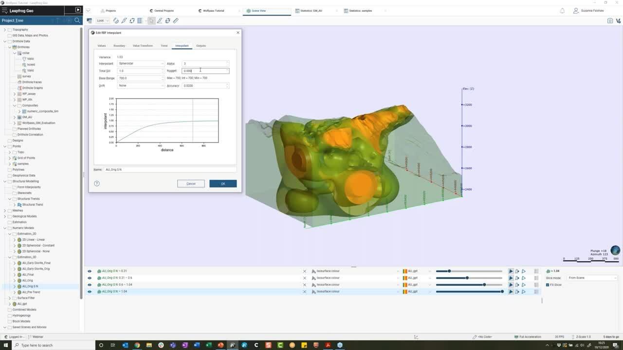
So if I go back now and go back to my interplant tab

[00:18:15.870]
to sort of look at some of these other settings.

[00:18:20.924]
So far we know we want to limit the influence

[00:18:27.030]
of our known data to a certain distance,

[00:18:30.820]
and that it’s the distance reign

[00:18:33.020]
essentially controlling that correlation.

[00:18:37.230]
It’s reasonable, therefore that you’re going to want to,

[00:18:40.110]
you’re going to want to change the base range

[00:18:42.610]
to something more appropriate.

[00:18:44.720]
And if you don’t know where to start,

[00:18:46.170]
then a rule of thumb could be around twice

[00:18:49.680]
the drill hole spacing.

[00:18:51.240]
So in this case, let’s, that’s around 700,

[00:18:55.170]
which is appropriate for this project.

[00:18:59.350]
We also want to consider our nuggets and in leapfrog,

[00:19:04.000]
this is expressed as a percentage to our some.

[00:19:09.070]
Increasing the value of the nugget will create smoother

[00:19:13.640]
results by limiting the effects of extreme outliers.

[00:19:18.660]
In other words, we would give more emphasis

[00:19:21.972]
to the average grades of our surrounding values

[00:19:26.190]
and less on the actual data point.

[00:19:29.490]
It can basically help to reduce noise

[00:19:32.330]
caused by these outliers

[00:19:34.630]
or with inaccurately measured samples.

[00:19:39.090]
What value to use here is very much decided on a deposit

[00:19:43.420]
by deposit case.

[00:19:44.780]
And by all means, if you or someone else

[00:19:48.500]
in your organization has already figured this out

[00:19:52.030]
for your deposit, then by all means apply it here,

[00:19:55.570]
perhaps for a gold deposit like this.

[00:19:58.970]
Then a rule of thumb will be,

[00:20:02.280]
let’s say, 20 to 30% of the sales.

[00:20:05.410]
So let’s just take this down.

[00:20:07.170]
For example, it’s 0.2, which is going to be 20% of that.

[00:20:10.793]
So I have 10% might be more appropriate

[00:20:14.170]
for other metallic deposits or indeed known,

[00:20:17.400]
if you have a very consistent data set,

[00:20:21.560]
we’ve spoken about drift already,

[00:20:25.220]
but now that we are pressed the range of influence,

[00:20:29.430]
then it’s really our drift that comes into play.

[00:20:33.520]
Using known in this case is going to help

[00:20:37.220]
control how far my samples will have an influence

[00:20:41.409]
before the estimation to case back to Siri.

[00:20:46.329]
I’m not going to delve too much

[00:20:50.140]
into the other settings here.

[00:20:51.850]
You can always read about these

[00:20:53.410]
to your heart’s content online,

[00:20:56.250]
but the take home point really is that,

[00:20:58.720]
it’s the interplant the base range,

[00:21:03.320]
that percentage nuggets to the sill and drift

[00:21:07.840]
that will have the most material effects

[00:21:10.480]
on your numeric model.

[00:21:13.400]
Get these rights and you should be well on your way

[00:21:16.030]
to producing a very best model

[00:21:17.970]
that makes the best of your geological knowledge.

[00:21:21.060]
All right, now we’ve talked a little bit about

[00:21:24.460]
these interplant settings.

[00:21:27.310]
I thought it would be worth a quick run over

[00:21:30.706]
on the ISO surfaces.

[00:21:33.750]
So we can see all these,

[00:21:35.860]
as we expand out our new model objects,

[00:21:39.530]
we’ve got ISO surfaces

[00:21:41.520]
and then of course the resulting output volumes.

[00:21:45.420]
When we pick cutoffs in our outputs tab,

[00:21:50.020]
we are simply asking leap frog to define some boundaries

[00:21:54.047]
and space and your contours,

[00:21:56.990]
where there is the same consistent grade.

[00:22:00.520]
Essentially the iso surfaces perform the exact same task

[00:22:05.910]
as our geological surfaces do

[00:22:08.696]
when we’re geologically modeling.

[00:22:10.776]
But instead of building these surfaces ourselves,

[00:22:14.690]
we’re simply picking grade boundaries

[00:22:17.051]
that we want to see and leapfrog we’ll go

[00:22:20.330]
and build them for us.

[00:22:23.250]
It is this contour surface that,

[00:22:26.343]
that we’re seeing here in 3D.

[00:22:29.770]
And if we want to visualize a specific value,

[00:22:34.020]
then we can do so by updating the ISO values here

[00:22:40.760]
before I do that, let me just jump back

[00:22:44.850]
into the grid of points,

[00:22:46.980]
just to highlight this on a sort of simpler dataset.

[00:22:53.947]
So back in with my grid of points, let’s say for instance,

[00:22:58.810]
I now want to visualize a contour surface

[00:23:03.350]
with a greater two, then I can replicate that here

[00:23:07.612]
simply by setting some appropriate value filters.

[00:23:12.049]
And we can see that now

[00:23:14.520]
sort of finding all of these sort of values of two in space.

[00:23:18.746]
And these it’s this point that of course

[00:23:22.840]
is going to become our contour.

[00:23:27.900]
For the hikers amongst us

[00:23:29.401]
who are maybe used to seeing elevation contour lines

[00:23:32.550]
on a TD map.

[00:23:33.850]
This is the same principle,

[00:23:35.492]
except in the case of our gold model.

[00:23:38.180]
We’re simply looking at a value representation in 3D.

[00:23:43.060]
So let me go back to my gold model once again

[00:23:49.690]
and actually set some better ISO values for this deposit.

[00:23:57.710]
So am just going to go double click back in

[00:23:59.960]
and head over to the output tab.

[00:24:02.870]
So let’s just set a few, make a little bit more sense

[00:24:06.670]
than the ones that are put in as default.

[00:24:10.900]
So let’s say 0.5, 0.75.

[00:24:16.350]
Let’s do 1.25 and at 1.5, I think we’ll suffice.

[00:24:27.970]
The other thing that I’m going to do

[00:24:29.640]
is take down the resolution on my higher grades

[00:24:33.990]
to try and be as accurate as possible.

[00:24:38.190]
And remembering to know you might not have heard it,

[00:24:41.360]
but remembering my much earlier points

[00:24:43.650]
about matching this where possible

[00:24:46.010]
to the drill hole complicit lens.

[00:24:48.500]
So that’s why I’m sort of picking the six here.

[00:24:53.500]
There’s also the ability in this tab to clump output values,

[00:24:59.740]
the default assumption is that

[00:25:02.610]
nothing should fall low zero,

[00:25:04.320]
which is why we’re seeing that clump,

[00:25:07.151]
but you can always change that if need be likewise,

[00:25:11.440]
you can set different lower,

[00:25:14.710]
and indeed upper bounds in the value transform tab

[00:25:19.280]
to cap any values you may deem too low or too high,

[00:25:23.360]
but I’m not going to focus on that for now.

[00:25:28.110]
So let me just let that run

[00:25:37.030]
and again, in the magic of eight forklifts,

[00:25:42.510]
so have a look at, so what that has produced,

[00:25:46.940]
and again, we’re starting to see something visually

[00:25:50.630]
that perhaps makes more sense.

[00:25:52.710]
That makes more sense to us and to our gold boundaries.

[00:25:58.990]
Now, if I want to see more connectivity

[00:26:03.010]
between my drill holes, then aside from the base range,

[00:26:07.550]
I could use a trend for this.

[00:26:09.630]
Also the central shear zone, for example,

[00:26:15.720]
is no doubt playing a dominant structural control

[00:26:21.870]
on my mineralization.

[00:26:23.750]
Starting to see a lot of our high grades,

[00:26:25.490]
sort of following some sort of trend here.

[00:26:29.370]
So applying a structural trend should help

[00:26:32.400]
to account for any changes in the strength

[00:26:36.409]
and direction of continuity along this ridge.

[00:26:41.330]
I’ve already defined a structural trends for the shear zone.

[00:26:46.230]
I sort of put it as something like this for now.

[00:26:51.130]
However we could have caused always update this as need be.

[00:26:55.410]
Either way, this is a typical step to take.

[00:26:58.640]
Given that nature is very rarely isotropic.

[00:27:03.530]
So let me go and apply this structural trends to my model

[00:27:11.960]
and which I can do from my trend tab.

[00:27:17.790]
And I’ve only got the one in my project at the moment.

[00:27:20.220]
So it’s just that stretch or trend,

[00:27:25.240]
and let’s just let that run.

[00:27:34.000]
And again, in a fantastic here’s one I prepared earlier,

[00:27:43.430]
we can see what that has done

[00:27:45.370]
this definitely you can see how that trend has changed

[00:27:49.870]
there is weighting of points in space

[00:27:52.780]
to define that continuity along that ridge.

[00:27:57.550]
So though powerful and usually they’ll be applicable

[00:28:01.560]
certainly in our sort of metallic gold

[00:28:05.776]
or indeed any deposit.

[00:28:09.970]
So now that we’ve sort of run to this point,

[00:28:14.870]
it’s likely at this stage

[00:28:17.030]
that we’re going to want to hone in our mineralize domains.

[00:28:21.590]
I spoke earlier about the early diorites unit

[00:28:27.780]
having our containing our highest mean gold grade.

[00:28:31.650]
So let’s come full circle and create a numeric model

[00:28:36.439]
for just this for you also.

[00:28:41.430]
So let me clear the scene and let me cheat

[00:28:48.370]
by copying my last model

[00:28:51.640]
with all of its parameters into the new one.

[00:29:05.230]
And now we can go into that copy of our model

[00:29:11.880]
and start to apply reasonable premises here as well.

[00:29:16.750]
Now, the first thing we’re going to want to do is of course,

[00:29:20.060]
set some boundary at the moment

[00:29:21.470]
it’s just the exact same as the last one,

[00:29:25.900]
which is the extent of my geological model.

[00:29:30.760]
Say, let’s go in and set a new lateral extent.

[00:29:34.830]
And what I’m going to do is use the volume

[00:29:37.971]
for my geological model as that extends.

[00:29:41.290]
Say from surface, and then under my geological models

[00:29:48.370]
under the output volumes,

[00:29:50.200]
I’m going to select that early diorite.

[00:29:57.230]
Now, whilst that’s running.

[00:29:59.920]
Remember that what that is going to do

[00:30:02.960]
is first of all, constrain your model

[00:30:06.710]
to that unit of interest.

[00:30:08.340]
So this is my early diorite.

[00:30:12.530]
And it’s also just only going to use the values

[00:30:22.910]
that refer to this unit,

[00:30:26.320]
what to do with that initial surface filter set up.

[00:30:29.700]
We then of course,

[00:30:30.533]
want to go and review our interplant settings here

[00:30:34.120]
to check that they’re still applicable.

[00:30:35.693]
Now that we’ve constrained our data to one domain.

[00:30:40.740]
Let me say, let me go back and double click into this model.

[00:30:46.240]
And let’s just double check once again,

[00:30:47.788]
that our interplant settings make sense.

[00:30:52.570]
It’s probably going to be more applicable in this case

[00:30:58.635]
that where we have an absence of data.

[00:31:01.290]
So again, on the outskirts, on the extents of our model,

[00:31:08.460]
that perhaps we’re going to want to revert

[00:31:10.730]
to the mean of the grade in the absence

[00:31:13.610]
of any other information.

[00:31:16.110]
In which case, the best thing that we can do

[00:31:19.030]
is simply to update the drift here to constant.

[00:31:23.890]
Hopefully you remember from that grid of points,

[00:31:26.570]
how that is always going to revert to the mean of the data.

[00:31:31.200]
I think for now,

[00:31:32.740]
I’m just going to leave every other setting the same,

[00:31:35.460]
but of course we could come in

[00:31:37.630]
and start to change any of these,

[00:31:41.270]
if we wish to see things a little bit differently,

[00:31:44.340]
but for now, it’s that drift that for me

[00:31:47.070]
is the most important.

[00:31:48.570]
So again, let me rerun and bring in a final output.

[00:32:02.240]
And if I just make these a little less transparent,

[00:32:06.520]
you can hopefully see now

[00:32:08.230]
that whereas before we had sort of that those waste grades

[00:32:14.230]
coming in on this sort of bottom corner,

[00:32:17.260]
we’re now reverting to what?

[00:32:19.500]
To something similar of the mean and I think in this case,

[00:32:23.330]
if I remember rightly the mean is yeah, 1.151.

[00:32:29.272]
So we would expect to be kind of up in that sort of darker,

[00:32:33.130]
darker yellow colors.

[00:32:38.020]
At this point,

[00:32:39.620]
I’m going to say that I’m reasonably happy

[00:32:42.230]
with the models I have.

[00:32:44.720]
I would, of course, want to interrogate these lot further.

[00:32:47.900]
Maybe make some manual edits

[00:32:50.502]
or double check some of the input data,

[00:32:53.578]
but for the purpose of this talk,

[00:32:55.490]
I hope that this has gone some way

[00:32:57.910]
in highlighting which interplant settings

[00:33:01.090]
will most effectively improve your numeric models.

[00:33:04.984]
I appreciate that this is a very extensive topic

[00:33:08.450]
to try and fit into a shorter amount of time.

[00:33:10.550]
Please do keep your questions coming in.

[00:33:14.090]
In the meantime,

[00:33:15.130]
I’m going to hand over to James now,

[00:33:19.030]
to run us through the indicator RBF interplant tool.

[00:33:24.550]
<v James>Thanks, Suzanna,</v>

[00:33:25.730]
bear with me two seconds and I’ll just share my screen.

[00:33:28.850]
So a lot of the stuff that Suzanna has run through

[00:33:32.350]
in those settings, we’re going to apply now

[00:33:34.830]
to the indicator numeric models

[00:33:38.520]
indicating numeric models are a tool

[00:33:41.530]
that is often underused or overlooked in preference

[00:33:46.220]
to the RBF models,

[00:33:47.810]
but indicator models can have a really valuable place

[00:33:51.480]
in anyone’s workflow.

[00:33:53.870]
So I’ve got the same project here,

[00:33:55.910]
but this time I’m going to be looking at

[00:33:58.050]
some of the copper grades that we have in the project.

[00:34:02.120]
If I go into a bit of analysis initially on my data,

[00:34:06.310]
I can see that when I look at the statistics for my copper,

[00:34:09.968]
there isn’t really a dominant trend to the geology

[00:34:16.350]
and where my copper is hosted is more of a disseminated

[00:34:19.879]
mineralization that is spread across multiple domains.

[00:34:24.480]
If I come in and have a look at the copper itself,

[00:34:27.600]
what I want to try and understand

[00:34:30.170]
is what it would be a good cutoff to apply

[00:34:34.740]
when I’m trying to use my indicator models

[00:34:37.580]
and this case here,

[00:34:38.650]
I’ve had a look at the histogram of the log,

[00:34:42.470]
and there’s many different ways

[00:34:44.380]
that you can approach cutoffs.

[00:34:46.954]
But in this case, I’m looking for breaks

[00:34:49.440]
in the natural distribution of the data.

[00:34:51.640]
And for today, I’m going to pick one around this area

[00:34:54.600]
where I see this kind of step change

[00:34:56.593]
in my grade distribution.

[00:34:59.410]
So at this point here,

[00:35:00.900]
I can see that I’m somewhere between 0.28 and 0.31% copper.

[00:35:06.770]
So for the purpose of the exercise,

[00:35:09.950]
we’ll walk through today we’ll use 0.3 as my cutoff.

[00:35:15.051]
So once I’ve had a look at my data and I have a better idea

[00:35:18.210]
of the kind of cutoffs

[00:35:19.660]
I want to use to identify mineralization,

[00:35:23.020]
I can come down to my numeric models folder,

[00:35:26.720]
right, click to create a new indicator.

[00:35:30.710]
I’ll be up in turbulent.

[00:35:34.186]
The layout to this is very similar to the numeric modeling.

[00:35:39.010]
Again, you can see,

[00:35:39.843]
that I can specify the values I want to use.

[00:35:43.050]
I can pick the boundaries I want to apply.

[00:35:45.090]
So for now, I’m just going to use the title project

[00:35:48.700]
in all my data.

[00:35:51.420]
And if I want to apply my query filters,

[00:35:53.730]
I can do that here as well.

[00:35:56.086]
A couple of other steps I need to do,

[00:35:58.670]
because this is an indicator interplant.

[00:36:00.820]
I need to apply a cutoff.

[00:36:02.730]
So what I’m doing here is

[00:36:03.590]
I’m trying to create a single surface

[00:36:05.960]
in closing grades above my cutoff of no 0.3.

[00:36:11.840]
And for the purpose of time,

[00:36:13.240]
I’m also going to just composite my data here.

[00:36:16.490]
So that it helps to run,

[00:36:18.710]
but it also helps to standardize my data.

[00:36:22.770]
So I’m going to set my composite length to four

[00:36:26.400]
and anywhere where I have residual links, less than one,

[00:36:29.240]
I’m going to distribute those equally back through my data

[00:36:33.950]
can give it a name to help me identify it.

[00:36:37.350]
And we’re going to come back

[00:36:38.500]
and talk about the ISO values in a minute.

[00:36:43.520]
So for now, I’m going to leave my ISO value

[00:36:45.338]
as a default of no 4.5, and then I can let that run.

[00:36:52.460]
So what leapfrog does with the indicators

[00:36:55.580]
is it will create two volumes.

[00:36:58.090]
It creates a volume that is considered inside my cutoff.

[00:37:02.150]
So if I expand my model down here,

[00:37:06.440]
we’ll see there’s two volumes as the output.

[00:37:08.800]
So there’s one that is above my console,

[00:37:11.960]
which is this volume.

[00:37:12.960]
And one that is below my cutoff,

[00:37:15.890]
which is the outside volume.

[00:37:19.775]
Now, at the moment,

[00:37:20.690]
those shapes are not particularly realistic.

[00:37:23.560]
Again, very similar to what we saw

[00:37:25.330]
with Suzanna’s explanation initially

[00:37:28.720]
because of the settings I’m using,

[00:37:30.100]
I’m getting these blow outs to the extent of my models.

[00:37:35.020]
The other thing we can have a quick look at

[00:37:36.388]
before we go and change any of the settings

[00:37:38.940]
is how leapfrog manages the data

[00:37:42.550]
that we’ve used in this indicator.

[00:37:45.050]
So it’s taken all of my copper values

[00:37:46.850]
and I’ve got my data here in my models.

[00:37:49.340]
So if I track that on,

[00:37:54.503]
just set that up so you can see it.

[00:37:57.690]
So initially from my copper values,

[00:38:01.310]
leapfrog will go and flag all of the data

[00:38:04.230]
as either being above or below my cutoff.

[00:38:07.060]
So here you can see my cutoff.

[00:38:09.270]
So everything above or below

[00:38:12.420]
it’s then going to give me a bit of an analysis

[00:38:15.870]
around the grouping of my data.

[00:38:18.130]
So here you can see that it looks at the grades

[00:38:22.570]
and it looks at the volumes it’s created,

[00:38:25.060]
and it will give me a summary of samples

[00:38:28.870]
that are above my cutoff and fall inside my volume,

[00:38:32.477]
but also samples that are below my cutoff

[00:38:35.080]
that are still included inside.

[00:38:37.510]
So we can see over here,

[00:38:38.530]
these green samples would be an example

[00:38:43.010]
where a sample is below my cutoff,

[00:38:45.977]
but has been included within that shell.

[00:38:49.360]
And essentially this is the equivalent

[00:38:51.200]
of things like dilution.

[00:38:52.110]
So we’ve got some internal dilution of these waste grades

[00:38:55.130]
and equally outside of my indicator volume,

[00:38:59.210]
I have some samples here that fall above my cutoff grade,

[00:39:04.290]
but because they’re just isolated samples,

[00:39:06.240]
they’ve been excluded from my volume.

[00:39:08.610]
So with that data and with that known information,

[00:39:13.800]
I then need to go back into my indicator

[00:39:16.160]
and have a look at the parameters and the settings

[00:39:18.671]
that I’ve used to see if they’ve been optimized

[00:39:20.910]
for the model I’m trying to build.

[00:39:23.820]
What we know with our settings,

[00:39:25.880]
and again, when we have a look at the inside volume,

[00:39:29.840]
if I come into my indicator here,

[00:39:32.327]
and go and have a look at the settings I’m using,

[00:39:35.726]
then I come to the interplant tab.

[00:39:39.260]
And for the reasons that Suzanna has already run through,

[00:39:42.740]
I know when modeling numeric data

[00:39:45.950]
and particularly any type of grade data,

[00:39:48.020]
I don’t want to be using a linear interplant.

[00:39:50.544]
I should be using my splital interplant.

[00:39:54.157]
The other thing I want to go and look at change in is that

[00:39:57.380]
I don’t have any constraints on my data at the moment.

[00:40:00.410]
So I’ve just used the model boundaries.

[00:40:02.950]
So I want to set my drift to known.

[00:40:06.410]
So again, there’s more of a conservative approach

[00:40:09.060]
as I’m moving away from data

[00:40:10.207]
and my assumption is my grade is reverting to zero.

[00:40:16.860]
We can also come and have a look at the volumes.

[00:40:20.090]
So currently our ISO value is five.

[00:40:23.020]
So we’ll come and talk about that in a second.

[00:40:25.340]
And the other good thing we can do here is

[00:40:26.920]
we can discard any small volumes.

[00:40:31.130]
So as an example of what that means,

[00:40:33.670]
if I take a section through my projects,

[00:40:40.000]
we can see that as we move through,

[00:40:41.440]
we get quite a few internal volumes

[00:40:44.910]
that aren’t really going to be of much use to us.

[00:40:47.920]
So I can filter these out based on a set cutoff.

[00:40:52.690]
So in this case,

[00:40:53.523]
I’m excluding everything less than 100,000 units,

[00:40:57.540]
and I can check my other settings to make sure

[00:40:59.450]
that everything else I’m doing,

[00:41:00.720]
maybe I used the typography is all set up to run how I want.

[00:41:05.480]
Again, what Suzanna talked about,

[00:41:07.018]
was there any time that you you’re modeling numeric data

[00:41:11.055]
best practice would be to typically use

[00:41:14.180]
some form of trend to your data

[00:41:16.560]
so I can apply the structural trend here

[00:41:18.460]
that’s Susanna had in hers, and I can let that one run.

[00:41:24.400]
Now, when that’s finished running,

[00:41:27.700]
I’ve got my examples here.

[00:41:31.800]
So if I load this one on,

[00:41:36.320]
I can see the outline here of my updated model

[00:41:39.240]
and how that’s changed the shape of my indicator volume.

[00:41:44.810]
So if we come back out of my section, put these back on,

[00:41:54.160]
I can see by applying those,

[00:41:56.410]
simply by applying those additional parameters.

[00:41:58.270]
So changing my interplant type from linear

[00:42:01.060]
to splital adding a drift of known

[00:42:03.510]
and my structural trend,

[00:42:06.830]
I’ve got a much more realistic shape now

[00:42:08.620]
of what is the potential volume of copper

[00:42:12.460]
greater than 0.3%.

[00:42:17.320]
Now, the next step into this

[00:42:19.250]
is to look at those ISO values

[00:42:20.930]
and what they actually do to my models,

[00:42:23.900]
the ISO value and if we come into the settings here,

[00:42:28.322]
so I’m just going to open up the sentence again.

[00:42:31.030]
You can see at the end, I can set an ISO value.

[00:42:34.140]
This is a probability of how many samples within my volume

[00:42:39.280]
are going to be above my cutoff.

[00:42:41.830]
So essentially if I took a sample

[00:42:44.380]
anywhere within this volume,

[00:42:46.230]
currently there is a 50% chance that,

[00:42:48.690]
that sample would be above my no 0.3% copper cutoff.

[00:42:53.871]
So by tweaking those indicator ISO values,

[00:42:58.860]
you actually can change the way the model is being built

[00:43:01.760]
based on a probability factor of how many,

[00:43:07.110]
what’s the chance of those samples

[00:43:08.940]
inside being above your cutoff.

[00:43:12.020]
So I’ve created two more with identical settings,

[00:43:15.190]
but just change the ISO value on each one.

[00:43:18.710]
If we step back into the model as a on a section,

[00:43:26.640]
so here we can see our model

[00:43:28.600]
which going to take the triangulations off.

[00:43:30.960]
So we’ve got the outline.

[00:43:33.320]
So currently with this volume,

[00:43:36.650]
what I’m saying is that I have a 50% chance

[00:43:39.497]
but if I take a sample, anywhere in here,

[00:43:41.780]
it is going to be above my cutoff

[00:43:44.810]
can also change my drill holes here to reflect that cutoff.

[00:43:49.810]
So you can see here, no 0.3% cutoff.

[00:43:52.460]
So you can see on my drilling samples

[00:43:55.470]
that are above and below.

[00:43:58.840]
If I go into my parameters

[00:44:01.000]
and I change my ISO value down to no 0.3.

[00:44:06.060]
So we can have a look at the inside value on this one,

[00:44:10.790]
what this is saying and I just made some,

[00:44:12.890]
so you can see it as well.

[00:44:13.810]
It’s basically, this is a volume

[00:44:15.930]
that is more of a prioritization around volume.

[00:44:18.830]
So this could be an example.

[00:44:20.130]
If you needed to produce a mean case and a max case

[00:44:23.677]
and a mid case,

[00:44:25.150]
then you could do this pretty quickly by using your cutoffs

[00:44:28.620]
and using your ISO values.

[00:44:31.620]
So drop in an ISO value down to 0.3

[00:44:35.120]
is essentially saying that there’s a 30% confidence

[00:44:38.130]
that if I take a sample inside this volume,

[00:44:41.240]
it will be above my cutoff.

[00:44:43.240]
So you can see that changing the ISO value

[00:44:45.960]
and keeping everything else the same

[00:44:47.300]
has given me a more optimistic volume

[00:44:50.640]
for my indicator shell.

[00:44:53.180]
Conversely, if I change my indicator ISO value to 0.7,

[00:44:58.780]
it’s going to be a more conservative shell.

[00:45:00.660]
So here, if I have a look at the inside volume in green,

[00:45:06.150]
and again, maybe just to help highlight

[00:45:07.740]
the differences with these.

[00:45:11.100]
So now this is my, exactly the same settings,

[00:45:15.220]
but applying a ISO value.

[00:45:18.260]
So a probability or a confidence of 0.7.

[00:45:22.070]
And again, just to, for you to review the notes.

[00:45:24.730]
So increase in my ISO value

[00:45:28.640]
will give me a more conservative case.

[00:45:31.720]
This will be prioritizing the metal content,

[00:45:34.500]
so less dilution.

[00:45:36.520]
And essentially I can look at those numbers and say,

[00:45:38.720]
I have a 70% confidence that any sample inside that volume

[00:45:42.700]
will be above my cutoff.

[00:45:47.020]
So I say it very quickly,

[00:45:48.520]
and particularly in the exploration field,

[00:45:50.610]
you can have a look at a resource or a volume.

[00:45:53.700]
And if you want to have a look at a bit of a range analysis

[00:45:56.300]
of the potential of your mineralization,

[00:45:58.500]
you can generate your cutoff and then change your ISO values

[00:46:03.340]
to give you an idea of how that can work.

[00:46:07.220]
Once you’ve built these,

[00:46:08.090]
you can also then come in and have a look at the,

[00:46:10.050]
it gives you a summary of your statistics.

[00:46:12.830]
So if we have a look here at the indicator at 0.3,

[00:46:16.040]
I look at the statistics of the indicator at 0.7,

[00:46:22.254]
we can go down to the volume.

[00:46:24.840]
So you can see the volume here

[00:46:27.610]
for my conservative ISO value at 0.7

[00:46:31.900]
is 431 million cubic meters,

[00:46:34.640]
as opposed to my optimistic shell, 545.

[00:46:40.330]
You can also see from the number of parts.

[00:46:42.350]
So the number of different volumes

[00:46:43.840]
that make up those indicators shells in the optimistic one,

[00:46:48.310]
I only have one large volume,

[00:46:50.930]
whereas the 0.7 is obviously a bit more complex

[00:46:54.520]
and has seven parts to it.

[00:46:57.314]
The last thing you can do

[00:46:59.190]
is you can have a look at the statistics.

[00:47:02.180]
So for example, the insight volume,

[00:47:04.720]
I can have a look at how many samples here

[00:47:06.970]
for below my cutoff.

[00:47:09.220]
So out of the what’s that 3,465 samples,

[00:47:15.260]
260 those are below my cutoff.

[00:47:19.200]
So you can kind of work out a, again,

[00:47:21.613]
a very rough dilution factor by dividing

[00:47:24.100]
the number of samples that fall inside your volume

[00:47:28.310]
by the total number of samples,

[00:47:29.610]
which would bring your answer around

[00:47:31.020]
in this case for the 0.3 around seven and a half percent.

[00:47:37.580]
So it’s just, this exercise is really just to highlight

[00:47:40.610]
some of the, again, the tools aren’t necessarily

[00:47:43.162]
used very frequently,

[00:47:45.200]
but can give you a really good understanding of your data

[00:47:48.930]
and help you to investigate the potential of your deposits

[00:47:53.200]
by using some of the settings in the indicator templates,

[00:47:58.669]
but ultimately coming back to the fundamentals

[00:48:02.620]
of building numeric models.

[00:48:04.870]
And that is to understand the type of interplant you use

[00:48:08.530]
and how that drift function can affect your models

[00:48:11.750]
as you move away from data.

[00:48:15.160]
So that’s probably a lot of content for you

[00:48:18.822]
to listen to in the space of an hour as always,

[00:48:23.500]
we really appreciate your attendance and your time.

[00:48:26.680]
We’ve also just popped up on the screen,

[00:48:28.580]
a number of different sources of training and information.

[00:48:33.810]
So if you want to go

[00:48:35.347]
and have a look at some more detailed workflows,

[00:48:38.440]
then I strongly recommend you look at the Seequent websites

[00:48:41.980]
or our YouTube channels.

[00:48:43.500]
And also in the, MySeequent page,

[00:48:45.930]
we now have all of the online content

[00:48:47.860]
and learning available there.

[00:48:50.110]
As always we’re available through the support requests.

[00:48:52.660]
So drop us an email

[00:48:54.057]
and if you want to get into some more detailed workflows

[00:48:57.820]
and how that can benefit your operations and your sites,

[00:49:01.830]
then let us know as well.

[00:49:03.570]
We’re always happy to support

[00:49:05.420]
via project assistance and training.

[00:49:08.900]
So that pretty much brings us to the end of the session

[00:49:13.290]
to the top of the hour as well.

[00:49:14.480]
So again, thanks to you for attending,

[00:49:17.780]
thanks to Suzanna and Andre for putting this together

[00:49:21.940]
and running the session.

[00:49:23.500]
And we’ll look to put another one

[00:49:25.700]
of these together again in the new year.

[00:49:27.690]
So hopefully we’ll see you all there.

[00:49:30.630]
Thanks everybody and have a good day.