Magnetic Surveying for anthropogenic objects: Data Processing

Good data processing is crucial to the successful completion of a magnetic survey. While often the quality of the processing relies on the experience of the data processor, there are a few rules we can follow to ensure we get good, repeatable results with every survey

Download the data set referred to in this webinar here.

Survey data provided courtesy of Geometrics, Base station data provided courtesy of Honolulu Magnetic Observatory: U.S. Geological Survey.

Overview

Video Transcript

[00:00:01.700]
<v Becky>Hi, everyone.</v>

[00:00:02.533]
Welcome to the third and final webinar

[00:00:04.930]
in our three-part series

[00:00:06.710]
on Magnetic Surveying for Anthropogenic Objects.

[00:00:10.050]
Today, I’m going to focus on processing the data

[00:00:12.740]
with Oasis montaj.

[00:00:14.380]
In case you missed it in the webinar description,

[00:00:16.860]
by signing up for this webinar series,

[00:00:18.660]
you have been given a two-week evaluation of Oasis montaj

[00:00:22.200]
with the geophysics and UXO extensions included,

[00:00:25.860]
both land and marine.

[00:00:28.270]
I’ve made the Hawaii dataset available for you to download

[00:00:31.470]
if you wish to follow along

[00:00:33.150]
or try it out on your own after this webinar.

[00:00:36.750]
This mini workshop is really just an introduction

[00:00:39.760]
to our tools.

[00:00:40.870]
And with the limited time available to us,

[00:00:42.830]
I will be moving quickly through the steps.

[00:00:45.130]
And I do skip a few of the easier things

[00:00:47.910]
that I think you can probably work out on your own

[00:00:51.030]
with our online tutorial.

[00:00:54.100]
The recording will be available shortly after the session

[00:00:56.550]
on the Seequent and Geometrics website

[00:00:59.030]
for you to review and practice on your own

[00:01:01.040]
if you wish to do so.

[00:01:03.120]
So today we’re going to start by importing the data.

[00:01:08.170]
We’re going to create a map, filter and remove some noise,

[00:01:11.610]
run a few corrections,

[00:01:12.780]
like the base station and background removal.

[00:01:15.830]
We’re going to look at gridding the data

[00:01:18.140]
and then picking targets.

[00:01:20.210]
If we have time, hopefully,

[00:01:21.330]
we’ll look at two different methods for picking targets,

[00:01:23.800]
dipoles and the Blakley method.

[00:01:30.200]
Yeah, so to start, if you don’t have a Seequent ID yet,

[00:01:35.760]
that’s the first thing you’ll have to do actually.

[00:01:38.090]
So you’re going to go to my.seequent.com.

[00:01:41.070]
And when you get to the Sign In page,

[00:01:42.730]
you’re going to click Create a Seequent ID.

[00:01:45.630]
Now, I do ask that if you want to use

[00:01:48.730]
the license that I assigned,

[00:01:50.500]
you need to register with the same email address

[00:01:52.870]
that you used for this webinar.

[00:01:54.700]
That’s the email address that I assigned

[00:01:56.720]
the evaluation license to.

[00:01:59.810]
Once you’ve signed up here,

[00:02:00.920]
you’ll be sent an activation email

[00:02:03.430]
where you’ll have to click on a link

[00:02:04.750]
to activate your account,

[00:02:06.310]
but then you’ll be able to come back here, sign in,

[00:02:12.970]
give it a second. (laughs)

[00:02:15.730]
Yeah, so yeah.

[00:02:17.030]
So once you’re able to sign in,

[00:02:19.750]
you’ll be able to view your license.

[00:02:21.460]
If you go to Subscriptions and click on My Subscriptions,

[00:02:24.430]
you’ll see the evaluation license, when it expires

[00:02:27.450]
and what extensions you have access to.

[00:02:30.220]
And if you go to Products,

[00:02:32.110]
you’ll be able to download and install Oasis montaj 9.10

[00:02:36.810]
from this link here.

[00:02:43.109]
All right, so let’s jump into the software now.

[00:02:46.610]
If you can open Oasis montaj,

[00:02:48.690]
this is the landing page where you can create a new project

[00:02:52.310]
or open an existing project.

[00:02:54.360]
So we’re going to create a new project

[00:02:56.270]
and we’re going to save it in the same folder

[00:02:59.020]
where we’ve put the raw data,

[00:03:01.986]
that XYZ file that I sent everybody.

[00:03:04.860]
And we’re just going to call it Hawaii, something simple.

[00:03:09.520]
It doesn’t really matter what this project is called.

[00:03:14.430]
So you can see along the top, it’s loaded our core menus.

[00:03:17.610]
These are the menus that come with Oasis montaj essentials.

[00:03:21.450]
So if you have no other extensions,

[00:03:23.240]
you can still do quite a lot with the software.

[00:03:26.640]
And these are also the similar tools that you get

[00:03:29.380]
with the new Oasis montaj Field version

[00:03:33.390]
that if you’re a Geometrics customer, you can get access to.

[00:03:40.470]
So that’s a very light version of Oasis montaj,

[00:03:44.240]
but it’s sort of similar to these core menus,

[00:03:48.400]
just a little bit of background there.

[00:03:52.780]
What we’re going to start with

[00:03:53.970]
is loading the menus that we want to use today.

[00:03:57.290]
So if you click on this Load Menus button,

[00:04:00.330]
you’re going to expand the Extensions section.

[00:04:03.310]
And I have a full license,

[00:04:05.540]
so you see there’s a lot more menus available.

[00:04:08.090]
But you should see Geophysics.

[00:04:10.840]
So you can load the Geophysics menu.

[00:04:13.250]
You should also see UXO Land and UXO Marine.

[00:04:16.320]
So we’re going to go ahead and just load both of those

[00:04:18.780]
or all three of those menus.

[00:04:21.520]
All right, so we’re going to start just by importing the data.

[00:04:25.840]
If you right click on Databases, you can click New Database.

[00:04:29.840]
And we’ll just call this,

[00:04:30.870]
again, we’re just going to call it Hawaii.

[00:04:33.340]
I’m going to just accept the default 200 lines, 50 channels

[00:04:37.060]
and click OK.

[00:04:39.780]
I’ve already done this once, so for me it says overwrite,

[00:04:42.730]
for you it should just have created the database.

[00:04:47.400]
So I’ve just double clicked it to make it full-screen here.

[00:04:50.290]
And just a little trick, if you have the XYZ file,

[00:04:55.440]
open here in your working directory

[00:04:59.580]
in this processing folder.

[00:05:01.880]
You can just click this XYZ file

[00:05:04.470]
and you can drag and drop it into the database.

[00:05:07.440]
And that’s actually going to just load it automatically.

[00:05:10.720]
So XYZ’s a really simple format to work with.

[00:05:16.950]
Okay, so we’ve imported the data, we have our coordinates,

[00:05:22.040]
we have both latitude, longitude, and x and y in UTMs.

[00:05:27.610]
It’s also…

[00:05:29.200]
No, it’s currently unknown.

[00:05:30.390]
So actually, the first thing we can do

[00:05:31.750]
is just set our coordinate system up.

[00:05:35.440]
So if you go to Coordinates, Set Coordinate System,

[00:05:38.640]
we’re going to assign it to WGS84/UTM zone 4N.

[00:05:54.610]
And I have it saved here as a favorite,

[00:05:56.630]
but if just type in 4N, for example,

[00:06:00.970]
you can scroll down here to World, Northern Hemisphere,

[00:06:07.950]
and it’s in this 162 to 156.

[00:06:14.570]
That sets our coordinate system,

[00:06:16.010]
and you can verify it

[00:06:17.100]
in the bottom right-hand corner down here.

[00:06:22.330]
I like to create a map right away

[00:06:25.160]
and visualize my line path.

[00:06:27.380]
I want to see what we’re actually looking at.

[00:06:29.590]
So once you’ve set the coordinate systems,

[00:06:32.300]
you can create your first map.

[00:06:34.220]
So I’m going to go up to the Map menu, New,

[00:06:37.530]
and I’m going to just click on Scan Data.

[00:06:39.660]
And so that looks at the minimum maximum x, y,

[00:06:43.620]
and fills in the blanks for us automatically.

[00:06:46.770]
So we’re going to click Next

[00:06:49.460]
and we’re just going to give it a name.

[00:06:50.640]
So again, I’m going to just call it Hawaii

[00:06:52.930]
and I’m going to leave the map template.

[00:06:54.970]
That’s just the page size.

[00:06:56.360]
If you were going to print this, you need to tell it here

[00:06:58.810]
what size page you want to print it on.

[00:07:01.960]
I’m going to click Scale.

[00:07:03.850]
It’s going to pick the minimum scale

[00:07:05.860]
that this data fits on this page.

[00:07:09.820]
And then I usually just round that up.

[00:07:11.470]
I like even numbers.

[00:07:13.020]
I’m going to say 7,500 here.

[00:07:15.510]
And make sure your coordinate system is correct

[00:07:17.867]
and click Finish.

[00:07:23.850]
That just creates this empty map for us.

[00:07:26.880]
And then I’m going to go to Line Path.

[00:07:29.060]
So that’s under Map Tools, Line Path,

[00:07:32.140]
and this is going to display for me

[00:07:35.830]
the path that the boat collected the data along.

[00:07:40.310]
So just because I know from experience,

[00:07:43.860]
I want to just make my labels a little bit smaller.

[00:07:49.060]
And there’s an option down here which says Break on Gaps,

[00:07:52.200]
and this means if there’s a gap,

[00:07:53.820]
what this does is it connects the dots.

[00:07:56.260]
So it just draws a straight line

[00:07:57.660]
from one data point to the next.

[00:08:00.790]
But this can be a little bit misleading.

[00:08:03.070]
If you actually have big gaps in the data,

[00:08:06.180]
it basically draws the line across it.

[00:08:09.640]
So if you want to actually be able to visualize gaps

[00:08:12.190]
that are greater than, let’s say half a meter,

[00:08:15.480]
you can just put in here

[00:08:17.030]
where you want multiple line segments.

[00:08:20.230]
So it’s going to connect the dots

[00:08:22.280]
for anything that’s smaller than half a meter.

[00:08:24.750]
And if it’s greater than a half a meter,

[00:08:26.170]
it’s actually going to show you in your line path

[00:08:28.500]
where that gap in the data is.

[00:08:30.960]
So let’s just put half a meter here.

[00:08:34.090]
Also for UXO, I tend to put the thinning resolution to zero.

[00:08:38.560]
This just means that for larger datasets,

[00:08:42.050]
to make it a little bit faster,

[00:08:43.920]
it can remove the amount of points it uses to define a line,

[00:08:49.770]
but for UXO, when we’re getting down

[00:08:51.440]
to the really nitty-gritty detail,

[00:08:53.810]
this can sometimes cause offset in where your data is

[00:08:56.950]
and where the line path is drawn.

[00:08:59.070]
But if we reduce this to zero,

[00:09:02.030]
the line path should match your points exactly.

[00:09:05.350]
It can slow your map down a little bit,

[00:09:07.700]
so just something to be aware of.

[00:09:11.230]
All right, so now we have our path,

[00:09:14.010]
and I don’t see any gaps in the data,

[00:09:16.000]
so that’s sort of like our first QC

[00:09:19.720]
to know that we don’t have any gaps

[00:09:21.950]
of half a meter or larger in this dataset.

[00:09:27.288]
I just kind of got OCD in me,

[00:09:30.620]
I like everything to look nice.

[00:09:33.320]
I want to actually put a base map on here,

[00:09:35.950]
I want a legend, a scale bar, things like that.

[00:09:38.880]
So we’re going to go to Map Tools, Base Map,

[00:09:41.430]
and we’re going to draw our base map.

[00:09:46.770]
If you wanted to change your scale,

[00:09:48.030]
you can do so at this stage when you draw your base map.

[00:09:51.530]
And then I’m just going to adjust my margins.

[00:09:54.610]
So I want to leave a gap at the bottom,

[00:09:56.670]
but I don’t need a bigger gap around each of the edges.

[00:10:00.140]
And then this inside data margin

[00:10:01.790]
is the amount of space you’re going to leave

[00:10:03.260]
between the data and the start of your maps around.

[00:10:06.800]
So if you actually want to see

[00:10:09.380]
what’s happening around your dataset,

[00:10:11.330]
so around this line path,

[00:10:12.950]
you can just increase these inside data margins.

[00:10:16.070]
And so this is an interesting area because it’s near shore.

[00:10:19.830]
Normally with these offshore surveys,

[00:10:22.790]
I don’t set this inside data margin to be very big

[00:10:25.770]
because there’s nothing to see but water.

[00:10:28.240]
But in this case, since we’re near shore,

[00:10:31.040]
we’re in the harbor actually,

[00:10:31.960]
I think it’s actually Pearl Harbor,

[00:10:34.700]
if we just increased that a little bit,

[00:10:36.260]
we can start to see the shore

[00:10:37.580]
and we can actually figure out

[00:10:39.700]
where we are exactly in Hawaii.

[00:10:43.750]
And so then we can click Next.

[00:10:47.340]
I have a bit of a standard here.

[00:10:49.100]
My maps, I select to gray for my UTMs.

[00:10:53.760]
And I always put my latitude longitude

[00:10:57.790]
as edge ticks only.

[00:10:59.440]
So that means the only lines I’m going to get on my map,

[00:11:02.470]
the coordinate grid is going to be the UTMs,

[00:11:05.180]
but I will still see where the lat longs are

[00:11:08.320]
just around the outside.

[00:11:12.020]
And then this is the simple title block.

[00:11:14.110]
So we’re just going to call this Hawaii.

[00:11:17.040]
This is a single mag dataset.

[00:11:19.460]
So we’re going to call it Single mag, maybe Total Field.

[00:11:24.230]
We’re using a G-882 Geometrics magnetometer.

[00:11:28.130]
This is actually a dataset from Geometrics.

[00:11:31.400]
So they provided this.

[00:11:34.030]
And yeah, it’s a total field magnetometer.

[00:11:39.560]
So maybe here, we can say,

[00:11:44.870]
you can put your name as the processor,

[00:11:47.850]
and then at the bottom you can put the date

[00:11:53.680]
and then click Finish.

[00:11:56.360]
And then on your map, you can click on this world button

[00:11:59.280]
and it will just take you to the full view of your map.

[00:12:03.980]
So that looks a little bit nicer.

[00:12:06.650]
We have some background images that you can add.

[00:12:09.310]
So if you go up to the Data Services menu,

[00:12:12.520]
and you click on Add Azure Maps Imagery,

[00:12:15.900]
this will give you a satellite image in the background.

[00:12:18.920]
So we can select Aerial and click OK.

[00:12:25.530]
And this is the image I was talking about where,

[00:12:30.070]
because we left that extra space around the data,

[00:12:33.090]
we can actually see parts of the land,

[00:12:35.790]
and we can see that we’re working inside this Harbor area.

[00:12:40.080]
On your map, if you just expand your map manager,

[00:12:44.060]
and then I like to pin it open

[00:12:46.110]
and then we click on that Full World button,

[00:12:50.760]
if you expand the data view and the base view,

[00:12:53.810]
this will just show you what layers you have

[00:12:56.080]
displayed currently on your map.

[00:12:58.080]
So I like to have this open at all times.

[00:13:00.850]
And the difference here

[00:13:02.640]
is that anything in the data view at the top here

[00:13:05.840]
is geo-referenced.

[00:13:07.290]
And so you don’t want to move

[00:13:08.720]
or reposition any of these layers.

[00:13:10.520]
And they should be locked so that it doesn’t let you.

[00:13:14.360]
And if you want to just adjust this aerial image,

[00:13:17.580]
you can highlight, you can select it.

[00:13:19.650]
And then there’s this transparency option down here.

[00:13:22.270]
So if we make it a little bit transparent,

[00:13:23.920]
we can actually see the line path on top of it.

[00:13:28.680]
Okay, so this just sort of sets the background.

[00:13:31.210]
One of the things we need to know for when we grid the data

[00:13:38.420]
is we need to know what the line separation is

[00:13:41.970]
in this dataset.

[00:13:43.310]
So if we just click this button here, which is Zoom to Box,

[00:13:49.120]
we can draw a box, a small box, over our line path.

[00:13:55.440]
And you can use your mouse roller to zoom in and out

[00:13:58.440]
just to adjust it a little bit.

[00:14:00.160]
But what I want to do

[00:14:00.993]
is I want to measure the approximate distance

[00:14:03.010]
between these lines.

[00:14:04.880]
So if you right click on your map,

[00:14:06.780]
you have this Measure Distance function.

[00:14:09.860]
And you can click on one point and then click on the next,

[00:14:12.303]
and you can see this is about 13 meters.

[00:14:15.660]
You can click Done, and then do it again.

[00:14:18.270]
Let’s measure somewhere down here.

[00:14:22.070]
That’s like 12 meters, eight meters.

[00:14:25.490]
So I think the idea here is that this was supposed to be

[00:14:28.790]
roughly 10 meter distance between lines.

[00:14:31.940]
You can see that they have quite a lot of variation

[00:14:34.360]
along their lines here.

[00:14:35.460]
So it wasn’t smooth sailing the whole time.

[00:14:40.410]
We can assume a 10-meter line separation.

[00:14:44.570]
So when we come to grid this data,

[00:14:46.760]
we can start with something

[00:14:47.960]
that’s roughly a quarter of that line separation.

[00:14:50.900]
So our cell size will be about 2.5 meters.

[00:14:58.040]
All right, let’s look at the database though.

[00:15:00.120]
Let’s look at the actual data

[00:15:01.210]
that we’re going to be working with.

[00:15:03.800]
In this database, there’s a few QC channels.

[00:15:08.340]
When you get the data in,

[00:15:09.720]
you might want to check out the mag first of all.

[00:15:12.110]
So we can right click on a number in the mag column,

[00:15:16.390]
and we can click Show Profile.

[00:15:20.116]
And that’s actually just going to give us

[00:15:21.120]
this graph of the data.

[00:15:24.440]
Another one that you’re going to look at is Signal.

[00:15:27.380]
So this is a really good QC channel.

[00:15:30.320]
We don’t use it to process,

[00:15:31.900]
we’re just using it to check

[00:15:33.840]
that we’re getting a good mag reading.

[00:15:37.420]
And so the higher the signal,

[00:15:39.830]
the better quality the data is.

[00:15:41.920]
If this signal drops below 500 or 200,

[00:15:47.900]
I think most of the time industry standard

[00:15:50.320]
is just to delete that data,

[00:15:52.080]
because it usually means there was a problem,

[00:15:55.930]
the mag values cannot be trusted,

[00:15:58.440]
maybe the magnetometer wasn’t oriented correctly.

[00:16:00.830]
It could have hit a dead zone,

[00:16:02.880]
or there was something wrong with it,

[00:16:04.720]
you’re not getting good signal.

[00:16:06.940]
And so you just want to really QC this

[00:16:10.300]
for any really low values.

[00:16:11.917]
And so you can do that by taking the statistics.

[00:16:15.360]
We can do it visually.

[00:16:16.430]
If you display it on a profile window like this,

[00:16:21.390]
you can use the arrows here to move up and down,

[00:16:24.270]
and we can inspect it.

[00:16:25.920]
And you can see here where the minimum values are,

[00:16:29.700]
but we can also take statistics.

[00:16:31.700]
So if I click on Signal, the name, three times,

[00:16:35.600]
I highlight the name and the data,

[00:16:37.690]
this means that when I say Statistics,

[00:16:40.090]
when I right click again and click on Statistics,

[00:16:42.880]
I’m going to be looking at the statistics for the data,

[00:16:47.530]
all the data on all the lines in this database.

[00:16:51.220]
If I had clicked twice and only highlighted the data

[00:16:54.550]
and not the name when I click Statistics,

[00:16:57.890]
I’d only be looking at the statistics for this line only.

[00:17:02.550]
So the signal channel on this line.

[00:17:05.210]
And so that’s just a little clue

[00:17:08.750]
as to what you have highlighted

[00:17:10.300]
and what statistics you’re taking.

[00:17:12.210]
So you can see here it says all lines

[00:17:14.610]
because I have everything highlighted.

[00:17:17.130]
And I can see that my minimum value is 449

[00:17:20.360]
and my maximum is 1500.

[00:17:22.410]
So depending on what your contract says,

[00:17:25.270]
if it’s 500, then there’s some values here,

[00:17:28.790]
and especially on this line right here,

[00:17:30.610]
that you might need to delete.

[00:17:36.386]
If it’s 200 or something a little lower

[00:17:38.560]
then you’re safe and this isn’t bad.

[00:17:41.320]
I don’t know what the standard is,

[00:17:42.950]
maybe that’s a good question

[00:17:45.350]
for Bart and Gretchen at the end.

[00:17:49.340]
I’ve seen different requirements for the signal value.

[00:17:55.020]
In this case, you can see that it’s actually very close

[00:17:57.360]
to what looks like an anomaly,

[00:17:59.230]
but if we just play the altitude channel,

[00:18:04.040]
you can see that they’ve just sort of skimmed the seabeds,

[00:18:10.590]
the altitude has gotten really, really low

[00:18:12.710]
right at this location.

[00:18:14.160]
So that probably has something to do with this signal.

[00:18:18.910]
Maybe it dipped or there was some really fast movement

[00:18:22.570]
and that caused a variation in that signal channel.

[00:18:25.750]
And so that probably means

[00:18:26.890]
that there’s something a little hinky about this anomaly.

[00:18:32.816]
It could just be a jerk,

[00:18:35.550]
the cable jerked or something like that.

[00:18:38.140]
We’d probably want to look at this

[00:18:39.460]
a little bit more carefully

[00:18:40.880]
and see what we could determine from this data.

[00:18:50.220]
We’re going to leave it.

[00:18:51.053]
We’re going to accept everything right now.

[00:18:53.080]
So what we want to do is, actually,

[00:18:55.340]
we’re going to use these arrows

[00:18:56.450]
and we’re just going to look through our data

[00:18:58.000]
and we’re going to see if there’s any problems

[00:18:59.760]
that we need to fix.

[00:19:01.550]
And I do believe there’s one spike that we need to clean up.

[00:19:05.990]
Yes.

[00:19:06.950]
So if we end up on line 18, you can see here,

[00:19:12.170]
there’s actually a spike in the data.

[00:19:15.530]
So we can see it in the altitude

[00:19:17.660]
and in the magnetometer channel.

[00:19:21.040]
So I’m going to right click in that top profile window,

[00:19:23.700]
and I’m going to click Zoom,

[00:19:25.260]
and I’m going to draw a little box over the base of that spike.

[00:19:29.950]
All right.

[00:19:32.069]
There’s a number of ways that you can get rid of this.

[00:19:34.980]
I’d like us to try using the nonlinear filter.

[00:19:37.400]
So it’s a really good filter

[00:19:39.450]
that captures these really sharp spikes in the data.

[00:19:43.810]
So we’re going to go to database tools, filters,

[00:19:46.320]
and we’re going to click nonlinear filter.

[00:19:52.210]
We’re going to select the mag channel.

[00:19:56.230]
And best practice here

[00:19:57.780]
is that you never edit your original data.

[00:20:04.424]
If you need to leave an audit trail.

[00:20:06.470]
If the customer that you’re delivering this database to,

[00:20:09.180]
they want to see everything you’ve done

[00:20:10.790]
to the original data.

[00:20:12.060]
That means, every time you run a filter

[00:20:14.240]
or you make a change,

[00:20:15.570]
you’re going to output a new channel name.

[00:20:18.360]
So in this case, I’m going to say Mag underscore edit.

[00:20:23.640]
So this is just the first edit.

[00:20:24.980]
It could be a manual edit, it can be a filtered edit.

[00:20:28.750]
It doesn’t really matter,

[00:20:29.583]
but this is usually what I call my D-spiked channel.

[00:20:34.390]
Now for the nonlinear filter,

[00:20:35.730]
it needs a width and a tolerance or amplitude.

[00:20:40.520]
What this is looking for is how many fiducials.

[00:20:43.650]
So this filter width is in fiducials.

[00:20:45.530]
And when I say the word fiducial,

[00:20:47.530]
what that means is, it’s a row number,

[00:20:50.580]
the number of rows or the number of samples.

[00:20:54.610]
So let’s cancel this ’cause we’re going to look at this spike

[00:20:57.980]
in a little bit more detail.

[00:20:59.390]
But it needs to know what is the width of the spike

[00:21:03.060]
that I’m going to delete that I want it to filter through

[00:21:06.160]
and what is the tolerance or what’s the amplitude,

[00:21:08.420]
so what’s the size of the spike.

[00:21:12.230]
I’m just going to cancel this for now.

[00:21:14.170]
And what I’m going to do is I’m going to highlight

[00:21:20.750]
the width in the profile window here.

[00:21:22.610]
And you can see that what I’ve highlighted

[00:21:24.790]
is three fiducials.

[00:21:26.810]
It looks like it’s only one fiducial,

[00:21:28.500]
but I always include one before and after.

[00:21:32.730]
So I would actually say that this is a three-fiducial spike.

[00:21:37.070]
And then the tolerance is basically the difference

[00:21:39.520]
between the background values and the actual spike.

[00:21:46.700]
So in this case, it drops down to 1,300 from about 35,000.

[00:21:51.770]
So we don’t need to be specific about this amplitude,

[00:21:56.470]
you don’t need to put the exact 35,000 minus 1300,

[00:22:01.050]
because it’s more general than that.

[00:22:03.800]
What we can do is we can give it something that’s smaller.

[00:22:08.776]
That’s almost 34 or 33,000.

[00:22:12.680]
That’s roughly 34,000.

[00:22:15.450]
We don’t need to put in 34,000

[00:22:17.500]
because we know that at a much smaller amplitude,

[00:22:20.810]
it would still be considered a spike.

[00:22:23.350]
So we could put something here like 5,000 nanoteslas.

[00:22:27.260]
And what we’d be saying is that,

[00:22:28.420]
if there’s a three fiducial anomaly

[00:22:32.400]
that has an amplitude of 5,000 nanoteslas, get rid of it.

[00:22:38.640]
And so you can capture many more spikes

[00:22:44.330]
by making it a little bit smaller,

[00:22:46.250]
and you can even make it wider.

[00:22:47.620]
So we could say even five nanoteslas.

[00:22:49.970]
If we have anomaly that’s five fiducials

[00:22:58.744]
that changes by 5,000 nanoteslas,

[00:23:00.640]
that would still be considered a spike

[00:23:02.490]
’cause there’s no UXO or object

[00:23:05.270]
that’s going to cause a change that rapid.

[00:23:09.220]
So let’s go back here to Filters, Non-linear Filter.

[00:23:13.300]
We’re going to select again the mag,

[00:23:15.400]
call it Mag underscore edit.

[00:23:20.900]
So let’s try that, five and 5,000.

[00:23:24.400]
And then we’re going to click OK.

[00:23:28.640]
Now it’s output this new channel.

[00:23:31.040]
So right away, what I’m going to do

[00:23:32.600]
is I’m going to right click on a number

[00:23:34.900]
under this new channel and click Show Profile.

[00:23:40.430]
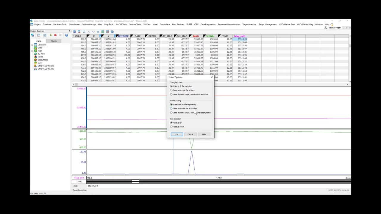
And it looks like there’s an offset,

[00:23:42.580]
but that’s really just because

[00:23:44.100]
we have to change our y-axis options.

[00:23:46.790]
So you’re going to right click in that profile window,

[00:23:49.470]
and you’re going to click, under Profile Scaling,

[00:23:53.130]
you want to select Same Access Scale for All Profiles.

[00:23:57.920]
And then you see that it shifts them

[00:23:59.790]
so that the y-axis is the same for the mag

[00:24:02.980]
and the mag edit channel.

[00:24:05.040]
And then I’m just going to zoom in again on the top here.

[00:24:08.350]
And you can see it’s drawn a straight line

[00:24:10.950]
just as we’d expected.

[00:24:12.670]
And to see it a little bit better,

[00:24:13.950]
if I actually just remove the original mag and rescale,

[00:24:19.490]
I can actually see where it used to be down here

[00:24:24.330]
and what it now looks like.

[00:24:25.750]
And it’s just basically drawn a straight line

[00:24:28.090]
through those three fiducials.

[00:24:34.970]
This dataset only had the one spike.

[00:24:38.819]
Normally you’d have to inspect each line

[00:24:40.410]
and make sure it did what you want it to do.

[00:24:43.140]
This is a really important step.

[00:24:45.890]
You need to make sure you’ve really cleaned it up.

[00:24:48.350]
This is really clean data,

[00:24:50.040]
so we don’t really need to do much to it.

[00:24:53.280]
You could filter it.

[00:24:54.420]
There’s small amounts of noise here and there,

[00:24:57.510]
but it’s really minor

[00:24:59.060]
and it’s not going to cause any significant difference

[00:25:01.210]
to our results whether we smooth it at this stage or not.

[00:25:04.600]
So we’re just going to carry on.

[00:25:07.340]
The next thing I want to do here is,

[00:25:10.960]
one of our participants in the previous webinar

[00:25:13.080]
asked me about a base station correction.

[00:25:16.130]
Now, generally off shore, we’re not running a base station

[00:25:19.960]
because we can’t get one close enough to our survey area

[00:25:23.520]
because the base station needs to be stationary, right?

[00:25:27.280]
There are some marine base stations, but they’re few,

[00:25:30.490]
and they’re few and far between let’s say.

[00:25:38.940]
The base station is not really generally done.

[00:25:41.550]
With this dataset, since we’re in Hawaii,

[00:25:44.100]
there is actually a magnetic observatory really nearby,

[00:25:48.890]
really close to the survey area.

[00:25:50.430]
And so just for the purpose of this exercise,

[00:25:53.240]
I’m going to run the base station correction

[00:25:55.100]
so that you can see how it’s done.

[00:25:58.590]
And so, actually, there is no base station tool

[00:26:04.080]
in the UXO Marine menu.

[00:26:05.960]
And that’s actually why I gave you the UXO Land tool.

[00:26:09.420]
Because if you go to Data Preparation for UXO Land

[00:26:13.610]
and you go to Data Corrections,

[00:26:15.290]
base station is the first correction that you’re going to do.

[00:26:19.200]
And so it is a lot more common

[00:26:21.140]
to see this correction done on land in UAV drone surveys,

[00:26:25.160]
or just land-based magnetic surveying.

[00:26:30.590]
All right, so we’re going to click this file, this tool.

[00:26:34.950]
And it’s looking for a couple of things here.

[00:26:37.820]
So first of all, it’s asking us for our survey database.

[00:26:40.277]
So that’s the only database we have at the moment,

[00:26:42.610]
so it’s Hawaii.gdb.

[00:26:45.210]
The date channel is just called date, time is called time.

[00:26:51.790]
And then it’s asking us for the input channel,

[00:26:54.180]
which is the mag channel that we want to actually correct.

[00:26:57.310]
So we’re going to use mag edit.

[00:27:02.780]
And you can actually save the base station.

[00:27:05.450]
So the base station file right now is a text file

[00:27:08.620]
that you should have in the zip file that I uploaded.

[00:27:18.165]
We’re going to go to base station.

[00:27:19.100]
So we’re going to load that base station file.

[00:27:23.332]
This is Honolulu, this is the date.

[00:27:28.054]
The magnetic observatory measures the field every minute,

[00:27:33.010]
so we have a once-per-minute reading.

[00:27:37.130]
You can click on this text file.

[00:27:41.040]
And then what you do is you select the first line

[00:27:43.600]
and then from the dropdown, you can tell it

[00:27:47.060]
which channel matches these fields, required fields.

[00:27:52.280]
So the mag-based field is actually this F.

[00:27:55.750]
Hon is for Honolulu field, I think.

[00:27:59.370]
So it’s at this Hon F.

[00:28:01.160]
The time field is just the time channel.

[00:28:03.760]
Date field is the date channel.

[00:28:05.970]
It’s asking us for the date format,

[00:28:08.030]
so that’s an that’s in year, month, day.

[00:28:12.100]
Now, this base station tolerance,

[00:28:14.740]
if your contract has a specification,

[00:28:18.700]
for example, for some surveys that says,

[00:28:22.527]
“You’re not to survey if the base station is reading,

[00:28:26.490]
if it’s changing two nanoteslas for every five minutes.”

[00:28:31.410]
So that could be one of your specifications.

[00:28:33.650]
So what this is asking us actually is,

[00:28:35.447]
“What is your tolerance in the contract?”

[00:28:38.880]
And it’s the unit is nanoteslas per minute.

[00:28:42.750]
So you’ll have to just work out to be what the…

[00:28:44.820]
If it says two nanoteslas per five minutes,

[00:28:47.360]
you just need to work it out what that would be per minute.

[00:28:50.460]
You put your tolerance in here,

[00:28:53.380]
and it will actually flag your data

[00:28:56.160]
where you shouldn’t have been surveying

[00:28:58.200]
because the base station tolerance is out of spec.

[00:29:02.090]
So this is actually a really nice simple step.

[00:29:04.070]
This saves you from having to import the base station

[00:29:07.040]
as a separate database and processing that.

[00:29:10.490]
So this should save you a lot of time.

[00:29:12.817]
It’s a really neat compact tool that does it all for you.

[00:29:16.580]
It also D-spikes your data.

[00:29:18.990]
So there is a filter here

[00:29:20.640]
that will get rid of all of the spikes of the database.

[00:29:23.550]
And that can happen

[00:29:25.120]
if you have somebody checking on your base station

[00:29:27.380]
while you’re surveying.

[00:29:28.960]
Often, when that person comes near,

[00:29:31.290]
if they have anything metallic on them,

[00:29:33.300]
you can see a little spike in the base station data.

[00:29:37.180]
So this tool will actually get rid of those spikes

[00:29:40.130]
so that you don’t…

[00:29:40.963]
Again, so it just saves you from having to do any processing

[00:29:43.920]
on the base station data.

[00:29:45.870]
And that’s it, so it should match everything up,

[00:29:48.970]
and it should give us…

[00:29:50.770]
Because we selected Save Interim,

[00:29:53.150]
we can see what the base station readings were

[00:29:55.410]
before it actually subtracted it from our survey data.

[00:30:01.270]
So let’s click OK.

[00:30:05.395]
And it’s going to run the correction.

[00:30:08.160]
And it’s giving us the mag edit base station corrected data.

[00:30:13.100]
And if we just load the hidden channel here,

[00:30:16.300]
this was the actual base station data.

[00:30:18.670]
So what it’s basically done is just subtracted

[00:30:21.650]
the overall base station reading from our survey reading.

[00:30:26.050]
And it’s left us with something

[00:30:27.190]
that looks a little bit like a residual,

[00:30:29.670]
although in this case it’s still quite a large number.

[00:30:32.710]
So the next step that we would do here

[00:30:34.650]
is a long wavelength removal.

[00:30:39.760]
But actually, just to see that difference,

[00:30:42.739]
let’s pause here and actually grid these results.

[00:30:47.560]
So I’m going to go to Grid and Image, Gridding,

[00:30:49.440]
Minimal Curvature.

[00:30:51.730]
We’re going to select our base, or diurnal corrected data.

[00:30:56.880]
And generally I just copy and paste that into my output.

[00:31:01.380]
And this is where we can actually select 2.5 meters

[00:31:04.880]
because that’s 1/4 of our line spacing.

[00:31:09.700]
Now, if you wanted the gridding

[00:31:12.140]
to actually reflect your footprint of your system,

[00:31:17.500]
you can adjust the blinking distance here.

[00:31:21.550]
So what I mean by that is,

[00:31:23.860]
if you’re doing something like a reconnaissance survey

[00:31:26.230]
where your lines are actually very far apart,

[00:31:30.120]
but you know that you only have a maximum detection range

[00:31:32.780]
of something like five meters,

[00:31:36.140]
you might only want to see a five meter swath

[00:31:38.510]
on either side of every line.

[00:31:42.220]
So you can put five meters in here and that will limit,

[00:31:48.080]
let’s say, the distance away from the line

[00:31:50.150]
that you’re greeting the data.

[00:31:52.000]
I’m going to use six meters in this case,

[00:31:53.810]
because there’s about a six-meter detection range.

[00:31:56.720]
They were flying at an average of four meters

[00:31:59.960]
above the sea bed,

[00:32:01.660]
and they needed to clear two meters below the seabed.

[00:32:05.450]
So the total detection range below the magnetometer

[00:32:08.560]
is about six meters.

[00:32:09.880]
And we know that on the surface

[00:32:12.770]
it’s a bit of like a semicircle.

[00:32:15.170]
So if it’s six meters below,

[00:32:17.170]
it’s six meters to either side as well.

[00:32:20.730]
We can set a six meter blinking distance,

[00:32:22.580]
so we’re going to get a total swath of 12 meters

[00:32:27.090]
for every line of data.

[00:32:30.974]
I’m going to click Finish.

[00:32:35.980]
So that’s given us this initial grid.

[00:32:39.090]
This is just a grid window, so you can see it has this GRD.

[00:32:42.250]
We can just close that.

[00:32:44.174]
I’m going to click on my map.

[00:32:46.910]
From the project explorer, I’m going to expand the grid layer.

[00:32:50.580]
I’m going to drag and drop my grid onto the map.

[00:32:56.390]
And then I’m going to use

[00:32:57.223]
just this Zoom to Full Extents button.

[00:33:01.790]
And that’s our first grid.

[00:33:03.560]
So I’m going to just turn off the line path.

[00:33:06.460]
So you can see that actually,

[00:33:11.110]
if they had a six-meter detection range,

[00:33:14.270]
they probably needed a little bit more coverage

[00:33:17.050]
in this dataset.

[00:33:18.340]
In reality, they probably had a much bigger detection range,

[00:33:21.240]
which is why this data was accepted and it’s actually okay.

[00:33:29.270]
But that’s fine, we can leave it like this.

[00:33:30.900]
This is actually really normal.

[00:33:32.070]
You will often see gaps in your data.

[00:33:36.270]
You will sometimes see gaps in your data and it’s real.

[00:33:39.180]
So that’s something you need to consider.

[00:33:41.200]
This can be areas where you can plant infills,

[00:33:45.220]
where you’re going to re-fly and collect more data

[00:33:47.900]
to fill in these gaps.

[00:33:50.740]
But what we’re seeing in this grid is a long wavelength.

[00:33:54.560]
So what we’re interested in

[00:33:56.440]
are these small discrete dipoles.

[00:34:01.070]
But what we actually see is this big, long wavelengths.

[00:34:05.200]
So you can see there’s a high on the left-hand side,

[00:34:07.800]
on the Western side of the grid,

[00:34:09.390]
and then the Northeast there’s this low.

[00:34:12.520]
This is part of a larger wavelength

[00:34:15.150]
that could be caused by geology

[00:34:17.290]
or something that’s just buried a lot deeper.

[00:34:23.692]
The next obvious step

[00:34:24.980]
is to remove that long wavelength from the data.

[00:34:27.570]
And that’s going to really bring out

[00:34:29.280]
and highlight these small discrete objects.

[00:34:33.950]
So let’s go back to our database,

[00:34:36.060]
and we’re going to run a background removal.

[00:34:40.170]
So if you go into the UXO Marine mag menu

[00:34:44.070]
and go to data corrections,

[00:34:45.930]
we’re going to do the background removal.

[00:34:49.850]
Now, the purpose of this background removal is, like I said,

[00:34:52.240]
to get rid of that long wavelength.

[00:34:54.360]
So we’re going to load in the base station corrected channel,

[00:35:00.800]
and we’re going to call it,

[00:35:03.340]
mag edit underscore base underscore background.

[00:35:09.800]
We’re going to do this in a couple of steps

[00:35:11.320]
so that you can see what the correction is

[00:35:14.410]
that we’re actually performing.

[00:35:17.920]
So I’m going to start with a nonlinear filter,

[00:35:20.200]
and I’m going to actually…

[00:35:21.250]
50 fiducials in this case works really well,

[00:35:26.270]
but I’m going to increase my tolerance

[00:35:27.820]
to about 10 nanoteslas.

[00:35:30.670]
And you’ll see the results in a minute

[00:35:34.090]
once we actually run this.

[00:35:35.950]
And that’s it.

[00:35:36.783]
So we’re just looking at the background first.

[00:35:40.550]
We’re trying to get an idea for what that really looks like.

[00:35:43.620]
So then I’m going to display the new channel.

[00:35:46.750]
So again, we’re going to right click on a number,

[00:35:48.420]
click Show Profile, and we’re going to look at this.

[00:35:53.220]
This is the actual background value

[00:35:55.430]
that we’re going to subtract from the original data.

[00:35:58.430]
And this is a good example here.

[00:36:00.520]
So what it’s done is,

[00:36:02.300]
everywhere where the green line matches the red line,

[00:36:05.490]
once we subtract the two, this is going to become zero.

[00:36:08.960]
And that’s really what we’re looking for.

[00:36:10.720]
We’re trying to isolate what we think are UXOs.

[00:36:14.630]
So over here on the left-hand side,

[00:36:16.330]
we have a really nice dipole.

[00:36:18.540]
So this is definitely something

[00:36:20.480]
that’s going to show up really well

[00:36:22.000]
after we remove this background.

[00:36:24.030]
And everywhere else, it’s just going to become zero.

[00:36:26.100]
And that looks okay.

[00:36:29.290]
On this line, same thing.

[00:36:30.820]
None of these really look like you UXOs,

[00:36:33.170]
but this could potentially be one.

[00:36:36.790]
These ones are probably a bit small and a little bit wide,

[00:36:39.530]
but after we subtract the green from the red,

[00:36:42.550]
we will be left with something that we can look

[00:36:44.850]
to see if it actually matches

[00:36:46.180]
what we’re looking for in our objects.

[00:36:49.500]
Now, the only thing is that this line,

[00:36:51.710]
because of the 10 nanotesla tolerance, is very noisy.

[00:36:57.702]
We’re going to run this again.

[00:36:59.080]
And actually, if you right click on the last channel,

[00:37:03.140]
you can re-run it from the right click menu.

[00:37:09.070]
So after we run this non-linear,

[00:37:10.790]
we’re going to run a baseline,

[00:37:12.390]
and that’s actually going to smooth the results for us.

[00:37:15.240]
So we’re going to run this at 0.8 smoothness and 0.2 tension,

[00:37:21.337]
and I’m going to click OK.

[00:37:22.820]
And it’s actually going to overwrite it,

[00:37:24.110]
so we should see right away the results

[00:37:27.160]
in our display channel.

[00:37:30.270]
There we go.

[00:37:31.103]
So that looks a little bit better.

[00:37:34.040]
So that second filter has really smoothed our results.

[00:37:38.060]
Now, one setting, one background calculation

[00:37:44.370]
will not always work for all lines.

[00:37:47.010]
So you do need to look at this really carefully,

[00:37:49.330]
and you’re going to see some that don’t look as nice.

[00:37:54.020]
For example, here, are these really UXOs?

[00:37:57.730]
We’re going to be left with small anomalies,

[00:38:01.870]
and you can see that it didn’t really draw a straight line

[00:38:03.890]
through them as we’d expect, or as we want to see.

[00:38:06.410]
So this is not a great fit.

[00:38:08.610]
And so I might actually use my line selection,

[00:38:11.790]
Select None, and then re-select just this line

[00:38:14.960]
and try to run a background correction

[00:38:16.730]
that better fits this individual line.

[00:38:20.000]
So this is a really, really important step

[00:38:22.060]
and it requires a lot of attention.

[00:38:24.880]
Unfortunately, there’s not really a faster way

[00:38:28.180]
that I know of at the moment.

[00:38:31.510]
It is what it is.

[00:38:32.930]
You just have to spend time on each line

[00:38:34.900]
and make sure you’re getting the best background removal

[00:38:39.450]
that you can get.

[00:38:40.660]
Like this one, this one’s not bad actually.

[00:38:42.480]
This is doing a pretty good job all the way along.

[00:38:47.970]
Yeah, this is okay.

[00:38:55.040]
For this workshop, we’re just going to leave it,

[00:38:57.180]
but in reality,

[00:39:00.290]
you will probably need to run more than one calculation.

[00:39:04.210]
So just be aware of that.

[00:39:05.850]
For example, like here, this is a really bad one,

[00:39:08.420]
because you’ll see that if we subtract

[00:39:10.000]
the green from the red,

[00:39:11.600]
it’s really going to cut short this anomaly and make it…

[00:39:14.760]
It’s going to give us two positives and a negative.

[00:39:19.210]
But really, I would expect this green line

[00:39:21.870]
to go across the base of this anomaly here.

[00:39:27.280]
The 50 probably wasn’t wide enough and we’d need to make it,

[00:39:31.120]
this might be like a 16 or a 70 width.

[00:39:35.130]
So we would rerun that background on this line

[00:39:37.600]
with a wider width.

[00:39:40.380]
But again, just for today, we’re going to accept it.

[00:39:42.380]
It looks pretty good on most lines.

[00:39:44.130]
It’s not perfect, but we’re going to move on.

[00:39:50.010]
So what we’re actually going to do now,

[00:39:51.830]
we’re going to go back to that same tool

[00:39:54.420]
and we’re going to click this button at the bottom,

[00:39:55.970]
which is Subtract the Background From Your Input.

[00:40:00.460]
And we’re going to change the output name to Residual.

[00:40:04.530]
So now we have an edited base

[00:40:07.040]
corrected residual mag channel.

[00:40:13.210]
And what you should see if we open a second profile window

[00:40:17.020]
is that it’s really centered around zero

[00:40:21.200]
except where we saw a difference

[00:40:23.030]
between the green and the red.

[00:40:27.530]
On some lines we’re left with these little anomalies,

[00:40:30.350]
and these probably are not UXO,

[00:40:32.440]
but we wouldn’t pick them when we do our target picking.

[00:40:36.570]
It’s fine that they’re there,

[00:40:39.650]
but we know that they’re probably not a UXO-like object.

[00:40:49.590]
This is one, this isn’t bad.

[00:40:50.800]
This might be actually picked

[00:40:52.130]
because it has a very big negative anomaly, negative dipole.

[00:40:57.270]
But yeah, so you can just kind of look through this

[00:40:59.420]
and see what the results look like.

[00:41:08.760]
Now that brings us to the last step,

[00:41:10.550]
which is picking targets.

[00:41:11.850]
So let’s grid this residual channel

[00:41:15.080]
and see how it compares to the other gridded image.

[00:41:18.990]
So we’re going to go back to Grid and Image, Gridding,

[00:41:20.930]
Minimal Curvature.

[00:41:22.770]
I’m going to grid the residual.

[00:41:25.610]
And again, I’m just going to copy and paste that

[00:41:27.410]
into my output.

[00:41:28.880]
I’m going to use the same cell size

[00:41:30.580]
and the same blinking distance.

[00:41:35.960]
And I’m going to, again, just close this

[00:41:38.360]
and I’m going to drag it onto my other map.

[00:41:44.390]
I don’t like looking at it with this color scale,

[00:41:46.550]
it’s showing a lot of noise.

[00:41:49.910]
So what I’m going to do

[00:41:50.900]
is I’m going to click on that grid in my map manager,

[00:41:54.130]
and I’m going to click the color tool,

[00:41:56.270]
and I’m going to use a normal distribution,

[00:41:59.170]
but I’m going to set the mean to zero,

[00:42:01.240]
so that means this yellow color

[00:42:04.020]
will be right on the zero mark,

[00:42:06.570]
and I’m going to increase my standard deviations.

[00:42:08.870]
I’m going to select something like 25.

[00:42:11.280]
And that means that really what I’m going to see

[00:42:13.310]
when I click OK here are just,

[00:42:16.225]
the high values are really going to stand out.

[00:42:22.940]
So these are the ones that I consider to be more UXO-like.

[00:42:28.070]
It’s just a really nice way of getting rid

[00:42:29.750]
of a lot of that very low-level noise in the data.

[00:42:34.430]
So now we can actually see

[00:42:35.660]
where some of these nice dipoles are

[00:42:37.350]
and what we actually might consider as UXO

[00:42:40.370]
or UXO-like object.

[00:42:46.170]
So from this, we can actually pick targets

[00:42:49.130]
using the dipole method.

[00:42:53.020]
We’re going to go to the UXO Marine mag menu,

[00:42:55.960]
and we’re going to click Pick Targets, Pick Dipoles.

[00:43:00.840]
No, it’s Find Magnetic Dipoles.

[00:43:05.210]
So we’re going to give it the input grid,

[00:43:06.830]
so that’s our residual.

[00:43:09.340]
And it’s asking us for a minimum positive peak.

[00:43:12.280]
Now these values will be different for every survey,

[00:43:15.860]
depending on what your height above the ground is

[00:43:18.560]
and what the object is that you’re looking for.

[00:43:21.420]
And really the only good way I have of determining this

[00:43:25.190]
is to do your surrogate item test.

[00:43:28.920]
And that’s where you put the object on the seabed

[00:43:31.410]
and you fly over it at different heights

[00:43:34.040]
before you start your survey.

[00:43:35.930]
And that’s because if you have a desktop study

[00:43:38.560]
and you know approximately what you’re looking for,

[00:43:45.078]
you can try to find an object

[00:43:47.410]
of the approximate same value.

[00:43:49.300]
And then at the different heights,

[00:43:50.500]
you can really see what the magnitude

[00:43:52.880]
of your anomaly will be.

[00:43:55.410]
And that’s going to help you decide

[00:43:57.250]
what these target picking parameters are.

[00:44:00.750]
And so that’ll be very different for every survey

[00:44:03.010]
and for every area based on the items

[00:44:06.000]
that you’re looking for

[00:44:07.200]
and based on your background values.

[00:44:09.510]
So if you’re in a very magnetically noisy area,

[00:44:13.490]
like I think the Baltic Sea

[00:44:15.160]
is a lot noisier than the North Sea,

[00:44:18.670]
you might need to fly a lot closer to the seabed

[00:44:21.550]
because you need your UXO to stand out

[00:44:25.940]
on top of the noise levels.

[00:44:28.240]
So again, those surrogate item tests,

[00:44:32.753]
you don’t just fly over the item,

[00:44:35.070]
you do background readings as well.

[00:44:37.450]
So you’re going to fly over a line where there’s no item,

[00:44:42.510]
and then you’re going to put the item down

[00:44:43.790]
and you’re going to go over it at different heights.

[00:44:45.960]
And that’s going to show you what the background levels are

[00:44:48.370]
and what it looks like with the object.

[00:44:52.810]
But anyways, for this survey,

[00:44:54.620]
we’re going to pick a minimum peak of 10 nanoteslas.

[00:44:59.210]
So what it does is it searches for the positive,

[00:45:00.920]
and then you give it a search radius in distance,

[00:45:04.160]
like in meters, around that positive

[00:45:06.490]
that it’s going to look for the negative.

[00:45:08.570]
So here, we’re going to put 25 meters.

[00:45:13.470]
And we’re going to save this in a new target database.

[00:45:16.930]
We’re going to call it Dipoles.

[00:45:20.770]
And then it’s going to create a dipole amplitude channel.

[00:45:23.130]
So this is the peak-to-peak value,

[00:45:25.870]
so from the negative to the positive.

[00:45:28.390]
And if we actually tell it what our survey database is,

[00:45:31.180]
it’s going to find the location of the target

[00:45:34.830]
on the closest line in our survey database.

[00:45:37.080]
So I really like selecting that option.

[00:45:40.061]
It’s not required though.

[00:45:41.840]
And then let’s click OK.

[00:45:48.677]
Okay, so here are the results.

[00:45:49.810]
And unfortunately it does change the colors.

[00:45:53.060]
There’s a little bug there that we need to fix.

[00:45:55.750]
So we’re going to put that back to zero and 25.

[00:46:01.150]
And you can see where it’s picked our dipoles for us.

[00:46:04.760]
So if I just zoom in on an area here,

[00:46:10.270]
you can see that it’s picked these dipoles.

[00:46:13.933]
So it’s showing you the black cross is the inflection point.

[00:46:19.850]
So that’s actually the location of the target

[00:46:22.400]
below the dipole.

[00:46:23.850]
And then it’s picking the most positive

[00:46:26.220]
and the most negative peak surrounding that.

[00:46:31.830]
So you can move around and you can inspect your results.

[00:46:38.378]
You can check that they make sense,

[00:46:40.190]
or if you need to tweak your parameters a little bit.

[00:46:44.660]
In the target database here,

[00:46:46.170]
you will get the location of the black cross,

[00:46:49.760]
so that’s the center of the dipole.

[00:46:52.640]
You’re going to get that dipole amplitude.

[00:46:54.580]
So that’s the peak-to-peak value.

[00:46:56.600]
You also get a length.

[00:46:58.560]
You get the closest line to that location.

[00:47:04.190]
So that’s from your survey database.

[00:47:06.110]
The distance along the line where it’s found,

[00:47:08.370]
and then the fiducials of the actual row it’s on.

[00:47:12.170]
And then we also give you a lot of information.

[00:47:14.750]
You also get the location of the positive peak,

[00:47:17.260]
the location of the negative peak.

[00:47:21.790]
But that’s it.

[00:47:22.623]
So that’s really all we have time for today.

[00:47:24.640]
I hope that was useful.

[00:47:26.840]
I’d really appreciate any of your comments or feedback.

[00:47:29.250]
And again, just to remind you,

[00:47:30.750]
you have your evaluation license for two weeks.

[00:47:34.260]
I’ve shared this dataset with you,

[00:47:36.210]
and you should be able to find this recording online

[00:47:39.720]
in a couple of days.

[00:47:40.770]
I’d say, give it at least a day and then check.

[00:47:44.250]
I don’t know when we’re going to get it up,

[00:47:45.500]
but we won’t wait too long.

[00:47:47.630]
And if you have any problems,

[00:47:49.200]
you can contact me directly,

[00:47:52.510]
or you can email [email protected].

[00:47:58.000]
We’ll be around afterwards.

[00:47:59.270]
Gretchen, Bart and I will be around afterwards

[00:48:01.420]
for any questions, but thanks very much.

[00:48:06.670]
<v Gretchen>Thank you, Becky.</v>

[00:48:07.820]
That was a really good training.

[00:48:09.990]
I personally enjoyed it.

[00:48:11.540]
I’ve had data I’ve had to process with Oasis montaj before,

[00:48:15.810]
and I wish I’d had you there to give me a hand.

[00:48:20.470]
I just wanted to mention that Geometrics and Seequent

[00:48:24.050]
are inviting you to be part of our early adopter program

[00:48:27.130]
to try out Oasis montaj Field for free for three months.

[00:48:31.520]
This special goes until April 29th.

[00:48:34.600]
It’s a free license to any Geometrics customer

[00:48:37.430]
who would like to try out the newest software offering.

[00:48:41.670]
Oasis montaj Field is a user-friendly prototype

[00:48:45.070]
that will still enable you

[00:48:46.180]
to visualize and perform on the spot quality control tests

[00:48:49.420]
or collected magnetic geophysical field data,

[00:48:52.440]
all within at the Oasis montaj environment.

[00:48:56.350]
It’s designed for people who are in the field

[00:48:58.690]
and aren’t looking to be weighted down

[00:49:01.190]
with every feature Oasis montaj offers,

[00:49:04.670]
but really those features that are special to them.

[00:49:08.000]
All right, thank you.

[00:49:10.980]
<v Becky>Thanks Gretchen.</v>

[00:49:12.760]
I see there’s a couple of people with their hands raised.

[00:49:15.780]
I’m not sure you’re going to be able to unmute yourself,

[00:49:19.220]
but if you want to type your question

[00:49:22.510]
in the question box.

[00:49:24.070]
So I think I see one now.

[00:49:30.680]
Let me look at that.

[00:49:32.830]
Sorry, one second. (giggles)

[00:49:39.520]
Right, okay.

[00:49:40.353]
So the first question in the chat was:

[00:49:44.550]
You chose UXO Marine Grad and UXO Marine Mag,

[00:49:47.660]
but is there any module for utility detection?

[00:49:52.690]
We don’t have a specific utility detection tool.

[00:49:56.180]
However, the picking targets that we did,

[00:49:59.120]
they won’t just work for discreet objects.

[00:50:02.860]
For example, if you run…

[00:50:04.720]
I used the dipoles, the dipole picking option,

[00:50:08.190]
but if you calculated an analytic signal

[00:50:10.930]
and used the Blakley method,

[00:50:12.770]
you can actually pick things that look like pipes.

[00:50:17.200]
There’s a couple of different settings

[00:50:18.660]
where you can pick discrete objects or you can pick ridges.

[00:50:22.260]
So if you see a ridge or a linear feature

[00:50:24.220]
in your magnetic data,

[00:50:26.270]
there is an option as part of the UXO target picking

[00:50:30.730]
that will let you pick those linear features.

[00:50:33.310]
And so that’s really what you can use

[00:50:34.630]
for cables and pipelines.

[00:50:36.290]
I’m not sure if there’s any other utility

[00:50:39.840]
that you’d be looking for.

[00:50:42.870]
I think we’ve actually been discussing

[00:50:44.770]
renaming UXO Marine UXO Land,

[00:50:47.440]
because the same tools can be applied for archeology,

[00:50:51.910]
for utilities and other things.

[00:50:55.500]
So it’s basically the same tools,

[00:50:57.821]
UXO Marine can be used

[00:50:59.030]
for any offshore near surface investigation, let’s say.

[00:51:06.900]
Okay, there’s another question here

[00:51:08.850]
about the altitude correction.

[00:51:10.660]
So the new platform, observation, altitude,

[00:51:12.890]
what value should be taken

[00:51:13.960]
for a very unstable altimeter values?

[00:51:16.810]
Yep, so that’s actually something

[00:51:18.010]
I didn’t really have time to get into very much.

[00:51:20.600]
We did a base station correction,

[00:51:24.530]
and we did a background removal,

[00:51:29.080]
but there is another tool

[00:51:30.460]
which will do an altitude correction.

[00:51:34.100]
If you have a really unstable altimeter values,

[00:51:38.230]
I would definitely run the altitude correction.

[00:51:40.640]
And then the new altitude that you use going forward,

[00:51:44.290]
so if you’re going to be calculating depths from that data,

[00:51:49.450]
all of your depths

[00:51:50.350]
would hang off of that new corrected altitude.

[00:51:54.160]
So you’d be correcting your altitude to a constant.

[00:51:57.070]
So if you said four meters,

[00:51:59.310]
that four meters becomes your new altimeter value

[00:52:02.950]
for the whole dataset.

[00:52:05.230]
Basically, once you do that altitude correction,

[00:52:07.070]
you’re kind of getting rid of the other altitude channel.

[00:52:13.220]
I hope that answers your question.

[00:52:17.820]
Another question here.

[00:52:18.700]
Is it possible to calculate depth

[00:52:20.530]
for discreet object or utility?

[00:52:23.260]
So, yeah, so again, we do have a couple of tools.

[00:52:25.520]
We have Euler deconvolution,

[00:52:27.070]
which will do depth to a discrete object or a pipe.

[00:52:31.180]
Again, the Euler deconvolution

[00:52:33.180]
uses something called the structural index,

[00:52:35.720]
and there is a structural index for linear objects.

[00:52:40.960]
So you can pick a structural index

[00:52:43.360]
for a pipe or a barrel.

[00:52:45.920]
So there’s a couple of different ones that you can use.

[00:52:47.920]
We also have something called potent queue,

[00:52:50.290]
which is a bit like an inversion style depth calculation.

[00:52:55.520]
And that’s also really good for pipes and cables.

[00:53:01.580]
And then, okay, another question here.

[00:53:03.810]
Although we didn’t cover Blakley method today,

[00:53:06.070]
I was wondering if there’s an easy way

[00:53:07.360]
to merge the target list by target locations

[00:53:10.880]
obtained from both the Blakley analytics signal

[00:53:13.770]
and magnetic dipoles.

[00:53:14.777]
It’s a really good question.

[00:53:16.250]
We do have a merge tool right now,

[00:53:18.850]
and I agree it’s not the greatest.

[00:53:21.110]
And it’s something we’re working on

[00:53:22.550]
for the next release.

[00:53:24.100]
So in the spring release, I believe,

[00:53:27.230]
we should have a new merge feature.

[00:53:29.320]
So I would say, hold on for now.

[00:53:32.480]
Let’s come back to that question.

[00:53:35.030]
There’s actually, well,

[00:53:36.600]
I know this was from somebody who uses UXO Marine.

[00:53:39.430]
There is a merge tool in UXO Land.

[00:53:41.850]
So while you have UXO Land for a couple of weeks now,

[00:53:44.970]
you could look at the merge tool

[00:53:46.970]
that’s available in UXO Land

[00:53:48.430]
’cause it’s a little bit better.

[00:53:51.030]
It has a couple more features.

[00:53:52.710]
So I think it might do a slightly better job

[00:53:56.150]
than the UXO Marine merge tool.

[00:53:59.370]
But we’re looking at ways also

[00:54:00.720]
where you could bring in something like a target list

[00:54:02.640]
from side scan sonar,

[00:54:04.200]
and you could cross-reference your targets

[00:54:06.530]
with your magnetic targets.

[00:54:08.890]
So this is something that we get asked a lot

[00:54:10.570]
and it’s something we’re trying to improve

[00:54:13.280]
how it currently works.

[00:54:18.134]
We have a few more minutes, so I’ll just keep going.

[00:54:19.710]
Questions are coming in fast and furious now.

[00:54:24.070]
How would you discriminate the autopicked target for UXO?

[00:54:28.860]
Yeah, so that’s another really…

[00:54:30.870]
That’s a hot topic, target discrimination.

[00:54:34.230]
So from magnetic data alone,

[00:54:37.520]
it’s really difficult to discriminate what you have.

[00:54:41.130]
So we don’t have a library

[00:54:44.320]
of magnetic signatures, for example.

[00:54:46.670]
If you were using EM, an advanced EM system

[00:54:51.050]
like the MetalMapper on land,

[00:54:54.500]
we have a library of signatures

[00:54:56.370]
that you would match the EM’s signature to.

[00:54:58.780]
And you can actually get a much better idea

[00:55:02.310]
on what’s clutter, or what’s garbage,

[00:55:05.600]
and what’s actually a known UXO.

[00:55:07.840]
With magnetics, we don’t provide you a library

[00:55:10.480]
because it’s too difficult.

[00:55:13.300]
We don’t have a list of what the signature looks like

[00:55:15.850]
at specific depths for specific UXOs.

[00:55:19.500]
I know that some people out there have been working on this,

[00:55:22.540]
and there’s a couple of third-party tools

[00:55:24.570]
that using magnetic moment and the depth and height

[00:55:29.990]
and et cetera, they do a bit of a better job.

[00:55:32.660]
So I think that’s an area

[00:55:35.130]
where you might just keep your eyes open

[00:55:36.870]
for new developments,

[00:55:38.090]
but at the moment we don’t have any discrimination tools

[00:55:40.620]
in Oasis montaj.

[00:55:42.170]
All that we can say

[00:55:43.003]
is that there is something magnetic there

[00:55:45.660]
and depending on how sharp it is and how big it is,

[00:55:48.300]
it could be a UXO.

[00:55:53.460]
Okay, another question.

[00:55:55.810]
The mag data was in the range of about 35,000,

[00:55:58.410]
but after the base station,

[00:55:59.790]
you plotted the difference of actual mag

[00:56:01.300]
and it was around 500.

[00:56:03.070]
Was that the corrected magnetic field?

[00:56:05.100]
So, yeah.

[00:56:07.420]
So our survey was reading around 35,000

[00:56:10.700]
and the magnetic observatory was around 34,500.

[00:56:18.430]
So when we subtracted it,

[00:56:19.560]
it left us with a residual of about 500.

[00:56:23.810]
I’m not really used to working so close to the equator.

[00:56:26.680]
I usually work in the 50,000 range up in the North Sea,

[00:56:31.870]
but yeah, we subtracted the actual,

[00:56:34.540]
the full values and that’s what it gave us.

[00:56:36.860]
So I hope I got the correct…

[00:56:41.890]
I did download it really quickly the other day

[00:56:45.320]
from the observatory.

[00:56:47.740]
It might be worth,

[00:56:49.290]
I don’t know exactly how far the observatory is

[00:56:51.880]
from our survey area.

[00:56:54.070]
And if we had actually put a base station

[00:56:57.240]
closer to the survey area,

[00:56:58.500]
we might’ve gotten slightly more accurate,

[00:57:01.430]
but I don’t think that that’s unusual.

[00:57:05.650]
But yeah, that is the corrected field.

[00:57:07.210]
And then after that we took the long wavelength removal

[00:57:10.310]
to get it down to zero.

[00:57:15.130]
Okay, another question.

[00:57:17.180]
I don’t know if we’re going to be able to answer

[00:57:19.040]
all the questions today,

[00:57:20.280]
but I will email you a response

[00:57:24.840]
if we don’t get to your question right now.

[00:57:26.840]
I think I’ll take probably just one more.

[00:57:36.472]
Here’s one.

[00:57:37.305]
What does it constitute to be a Geometrics customer?

[00:57:40.210]
I think that there’s actually…

[00:57:42.320]
What we’ll do, we’ll send a follow-up email

[00:57:44.500]
with the link to where you can sign up

[00:57:46.210]
for Oasis montaj Field.

[00:57:48.190]
And then I don’t know what checks they’re doing,

[00:57:50.310]
but you can register for it and see what happens.

[00:57:55.655]
And then there was a question here about the data.

[00:57:59.480]
Was it UXO total-field or gradient?

[00:58:02.300]
And this was a single magnetometer, but to be honest,

[00:58:07.690]
just because of the time we had today,

[00:58:09.970]
I took one magnetometer out of a TVG frame.

[00:58:15.370]
I can share afterwards if you’re interested,

[00:58:17.070]
the full dataset,

[00:58:18.420]
and it actually consisted of two magnetometers.

[00:58:20.970]
And that’s probably why we saw some gaps

[00:58:23.140]
in the gridded data,

[00:58:24.460]
because there really was another set of lines.

[00:58:28.200]
We didn’t have time today

[00:58:29.640]
to look at the full gradient processing,

[00:58:32.700]
that’s a much more involved processing sequence.

[00:58:36.730]
So I took just a single total field magnetometer

[00:58:39.530]
and showed you the workflow.

[00:58:43.280]
But to be honest,

[00:58:44.960]
that survey is actually a gradient survey

[00:58:47.530]
using the TVG frame and two G-882s.

[00:58:52.050]
You can find that data with the two magnetometers,

[00:58:54.360]
if you wanted to play with that

[00:58:55.810]
and try to process the full gradient.

[00:59:00.600]
Okay.

[00:59:01.433]
So I think that’s all we have time for today.

[00:59:03.210]
Thank you so much for your questions

[00:59:04.800]
and for coming to one or all three of them,

[00:59:09.460]
if this is the third one that you’ve watched.

[00:59:12.230]
The recordings will be available

[00:59:13.860]
on the Geometrics YouTube channel,

[00:59:15.960]
as well as on the Seequent community video page.

[00:59:20.880]
I’ll talk to our marketing department

[00:59:22.420]
and we’ll try to get it up tomorrow

[00:59:23.740]
so that if you wanted to replay this one with the data

[00:59:27.680]
and your evaluation license,

[00:59:29.470]
you have the full two weeks.

[00:59:31.490]
Your licenses will expire two weeks from yesterday.

[00:59:35.810]
So you have two weeks minus a day.

[00:59:40.450]
All right.

[00:59:41.283]
So thanks again and enjoy the rest of your day, everyone.