Leapfrog Works – Contaminants Extension Technical Webinar Series

 

This 4-part technical webinar series is designed for you to learn how to bring contaminant data directly into your Leapfrog Works 3D geological models and characterise, visualise, and create auditable estimates of contaminant mass and location in land and groundwater environments. Sessions 2-4 include a live Q&A at the end.

Webinar Data

• If starting at Session 1: Chlorinated Landfill Plume Webinar Data
• If starting at Session 2: Chlorinated Landfill Initial Project

Session One:

• Introductory video: Leapfrog Basics – Importing data and building a model

Video Transcript

[00:00:01.190]
<v Jeffrey>Hello, and welcome to the first</v>

[00:00:02.550]
of a four-part webinars series where we highlight

[00:00:04.900]
the workflow of the contaminants extension.

[00:00:07.920]
My name is Jeffrey McKeon,

[00:00:09.260]
a project geologist with Seequent out of Denver,

[00:00:12.350]
and I will be leading you through this workflow.

[00:00:17.660]
So in this initial webinar,

[00:00:19.790]
we are going to discuss how to import data.

[00:00:23.730]
We’re going to import a variety of data including maps,

[00:00:27.470]
GIS vector data, lithological data, contaminant data,

[00:00:30.383]
as well as an elevation grid.

[00:00:33.890]
We are then going to validate our data in Leapfrog Works

[00:00:37.630]
in order to standardize it for use

[00:00:39.600]
and downstream modeling processes.

[00:00:42.430]
We will then build a geological model

[00:00:44.730]
representing our lithological units

[00:00:46.616]
using our borehole interval data.

[00:00:49.930]
Then we will build a water table model

[00:00:52.670]
using the GIS vector data and borehole data.

[00:00:57.290]
Before jumping into the modeling process,

[00:00:59.480]
I just wanted to highlight the input data

[00:01:03.030]
that we are going to use for this project.

[00:01:06.680]
So that is located in this folder here on my computer.

[00:01:10.090]
So we have an aerial photo,

[00:01:11.550]
which is just an aerial map as a TIF file.

[00:01:14.920]
We then have our borehole information.

[00:01:16.700]
So we have our collar, contaminant intervals,

[00:01:20.060]
and our geology intervals as a CSV file.

[00:01:24.730]
We also have our topography as a MESH file

[00:01:28.030]
and our water table as a shapefile.

[00:01:32.040]
I just wanted to touch on the borehole tables.

[00:01:35.930]
So our collar table is composed of a hole ID,

[00:01:42.110]
an XYZ, our Easting, Northing, and elevation,

[00:01:47.650]
as well as max depth.

[00:01:51.150]
Our geology table is the hole ID,

[00:01:54.830]
from, to, and the geology interval.

[00:02:00.990]
And then our contaminant interval table is our hole ID,

[00:02:04.670]
from, to, and then our contaminant analytes.

[00:02:12.640]
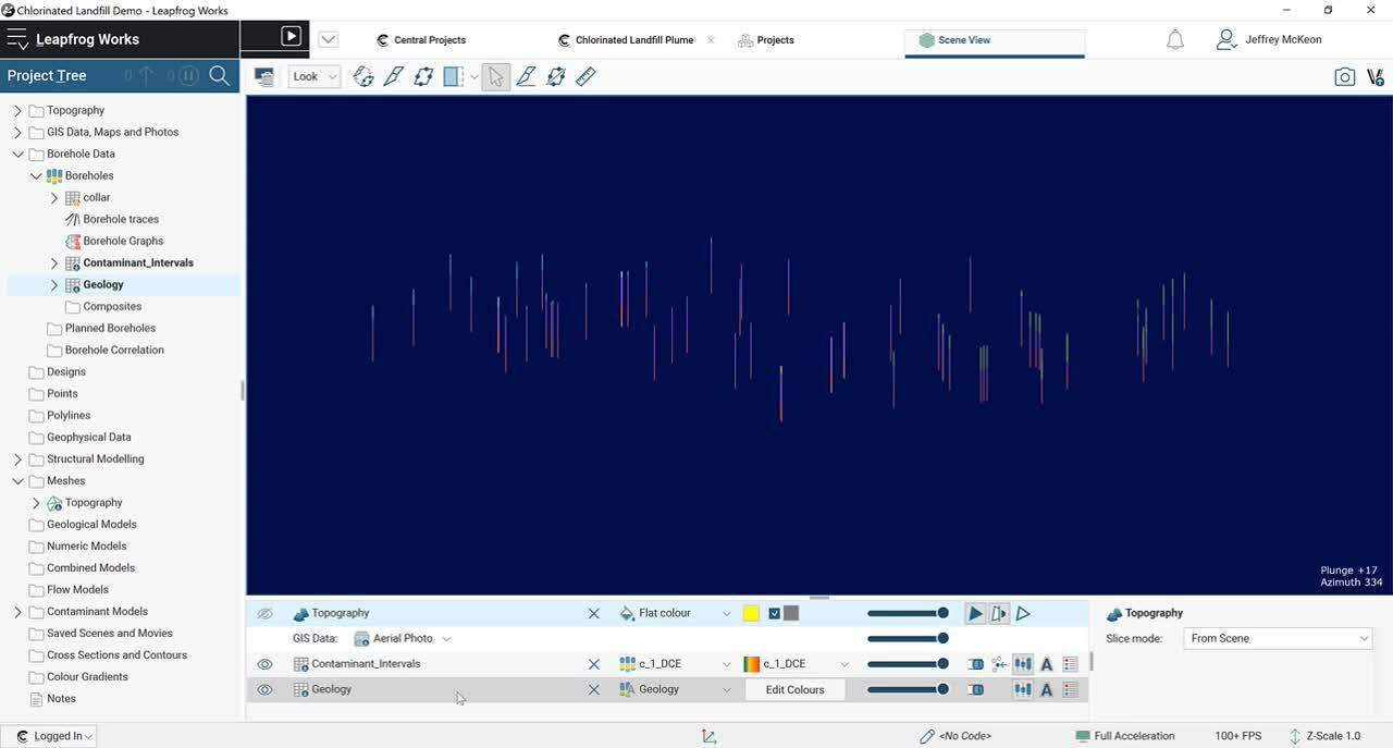
So now jumping into Leapfrog Works.

[00:02:15.840]
This is the interface of Leapfrog Works.

[00:02:18.090]
It’s split up into three different components.

[00:02:20.810]
You have your project tree,

[00:02:22.360]
which is where all of your data is housed.

[00:02:25.510]
You have your scene view,

[00:02:26.860]
which is where you visualize your data in the 3D space

[00:02:30.310]
and the shape list, which is anything that is visualized

[00:02:34.660]
in your scene view will appear here

[00:02:36.253]
just so you can keep track of what you are viewing.

[00:02:41.320]
Jumping into the project tree,

[00:02:44.142]
the project tree was built in a top-down approach.

[00:02:48.360]
It is workflow oriented.

[00:02:50.060]
So at the top you have your typography

[00:02:53.090]
and all of your inputs like your GIS data, borehole data,

[00:02:59.440]
points, polylines, geophysical data.

[00:03:02.380]
Moving downward into what you build

[00:03:03.980]
in Leapfrog Works being your geological models,

[00:03:06.650]
numeric models, contaminant models.

[00:03:10.040]
Moving further down, then you have your saved scenes

[00:03:13.930]
and your cross sections.

[00:03:15.860]
I’m going to discuss most of these folders

[00:03:19.270]
starting at the top.

[00:03:21.630]
So, first we’re going to build our typography.

[00:03:25.570]
Typography can be built from elevation grids,

[00:03:28.680]
from a surface, from GIS vector data, as well as points.

[00:03:32.380]
In this case, we have a surface.

[00:03:34.100]
So, first I need to load that surface

[00:03:36.906]
into the appropriate folder.

[00:03:39.270]
So I’m going to right click on Meshes, select Import Mesh,

[00:03:45.250]
and select my typography mesh.

[00:03:49.840]
I am okay with the default settings,

[00:03:51.770]
so I’m going to go ahead and click OK,

[00:03:55.020]
and that will start the import process.

[00:03:58.190]
In Leapfrog if something is importing

[00:04:00.240]
and you want to see where it’s at in the processing,

[00:04:03.213]
or just anything that’s processing in Leapfrog,

[00:04:06.130]
you can click this

[00:04:07.010]
and you can see what exactly is processing.

[00:04:11.970]
And once it’s done processing, this box will turn black.

[00:04:15.170]
We can see that there’s nothing processing now,

[00:04:17.910]
meaning our typography has successfully loaded.

[00:04:21.280]
We now need to take this input file

[00:04:25.650]
and build our topography from it.

[00:04:28.010]
So I’m going to right click New Typography, From Surface

[00:04:33.220]
and then select the surface that I just imported.

[00:04:36.350]
Click OK.

[00:04:38.170]
I’m okay with naming it topography.

[00:04:42.270]
And again, it’s done processing,

[00:04:47.800]
and now we can pull this into the scene.

[00:04:51.610]
To view anything in the scene,

[00:04:53.040]
all you do is click and drag and drop,

[00:04:55.920]
and then it will appear in your scene view.

[00:04:59.280]
And like I said, anything viewable,

[00:05:01.556]
anything that is in your scene view will appear

[00:05:04.690]
in the shape list down here.

[00:05:08.320]
So now that we have our topography,

[00:05:09.830]
I want to drape a GIS map onto my typography.

[00:05:17.270]
So first I need to load that into the appropriate folder.

[00:05:21.130]
So again, to import anything, you right click.

[00:05:24.900]
I’m going to import map.

[00:05:27.870]
So this specific map is already geo-referenced,

[00:05:33.500]
but I just want to note that you can geo-reference images

[00:05:39.440]
in Leapfrog Works as well.

[00:05:43.920]
So once my map is loaded,

[00:05:45.500]
if I want to drape either the map

[00:05:48.530]
or any of the GIS vector data that I have imported,

[00:05:53.290]
I’m going to come into my shape list.

[00:05:55.620]
And underneath my typography,

[00:05:57.010]
you can see this GIS data little drop-downs.

[00:06:00.620]
I’m going to click that, go to maps and photos,

[00:06:03.810]
and select the map that I just imported.

[00:06:08.070]
And here we can see that that was successful.

[00:06:14.670]
So now that I’ve imported my typography,

[00:06:16.690]
I’m going to move on to import some borehole data.

[00:06:21.690]
So again, to import anything into these folders,

[00:06:25.460]
you just right click.

[00:06:27.250]
With boreholes, we have the ability to import a local file

[00:06:30.150]
like a CSV, text file, or DAT file.

[00:06:33.494]
We can also import via Central,

[00:06:36.700]
which is sequence cloud-based data management software.

[00:06:41.560]
We can import via an ODBC like Access.

[00:06:45.580]
We also have the ability to connect to gINT,

[00:06:49.450]
and then you can also import via OpenGround Cloud,

[00:06:53.740]
which is Bentley’s cloud-based

[00:06:57.540]
geotechnical database software.

[00:07:01.020]
In this instance, I have a local file.

[00:07:03.080]
So I’m going to select import boreholes,

[00:07:05.740]
click on this little folder, and select my collar table.

[00:07:10.760]
I’m going to press Open.

[00:07:13.030]
We can see here

[00:07:13.863]
that it automatically pulled my geology table.

[00:07:16.690]
So I just need to add my contaminant interval table.

[00:07:21.927]
In this project, we don’t have a survey survey table,

[00:07:24.730]
because all of the holes are vertical.

[00:07:27.450]
You can also import downhole points in this initial import.

[00:07:32.350]
Once I’m happy, I’m going to click Import,

[00:07:35.100]
and it’ll bring up this screen.

[00:07:37.100]
This is just where you map the columns in the CSV file.

[00:07:43.630]
So we can see here that Works

[00:07:46.280]
has automapped these correctly, hole ID,

[00:07:49.950]
East, North, elevation, and max depth.

[00:07:54.690]
This has also automapped correctly hole ID,

[00:07:58.060]
from, to, geology.

[00:08:02.930]
For the contaminants interval,

[00:08:05.380]
I just need to designate these as one of these data types.

[00:08:11.630]
So I’m going to map these as numeric.

[00:08:13.700]
This is really important

[00:08:14.850]
if you want to use these as numeric values

[00:08:18.430]
in your modeling process,

[00:08:21.370]
especially for numeric models

[00:08:22.990]
and the contaminants extension.

[00:08:25.370]
So I’m going to map these as numeric values.

[00:08:33.690]
And once I’m happy with that, I’ll select Finish.

[00:08:38.560]
And then that will put these in my borehole table.

[00:08:45.150]
So we can see here initially that one of them has

[00:08:48.770]
a little red circle with an exclamation point,

[00:08:51.790]
and one has a little yellow triangle

[00:08:55.470]
with an exclamation point.

[00:08:57.020]
That means that there are errors in these files.

[00:09:02.040]
So to jump into our modeling process,

[00:09:06.260]
we need to fix these or else they won’t be usable.

[00:09:09.600]
So we can see here,

[00:09:10.450]
I just dragged the contaminant interval data into the scene,

[00:09:14.070]
and we can see that there’s very limited data.

[00:09:21.820]
All of our analytes aren’t mapping correctly.

[00:09:24.130]
So this is not usable.

[00:09:25.420]
So we need to fix this

[00:09:26.330]
before we jump into the modeling process.

[00:09:29.080]
To do this, I’m just going to right click

[00:09:31.070]
and select Fix Errors,

[00:09:33.340]
and that’s going to bring up this table,

[00:09:35.840]
so we can see that there’s some invalid depths

[00:09:39.380]
and some invalid values handling.

[00:09:42.140]
I’m going to jump into this one first, starting with total.

[00:09:47.640]
So we can see here that this is broken up

[00:09:49.890]
into three different parts.

[00:09:52.110]
We have missing values.

[00:09:53.470]
So this defaults to omit these missing intervals,

[00:09:56.880]
which I am okay with.

[00:10:00.240]
Non-numeric values, we can see that the default action

[00:10:03.830]
is to omit these as well.

[00:10:06.440]
I’m going to want to use these.

[00:10:09.350]
We can see in this right hand column

[00:10:12.860]
that these are the non-numeric values.

[00:10:16.090]
So a lot of times when a value is below the detection limit,

[00:10:20.510]
they say that it’s less than the lower detection limit.

[00:10:27.698]
Leapfrog can’t use this as a numeric value,

[00:10:30.070]
because this symbol is not numeric.

[00:10:33.790]
So what we are going to need to do is replace this with…

[00:10:37.540]
And whenever I see this,

[00:10:38.520]
I just do half of this detection limit.

[00:10:40.580]
So I’m going to do 0.05.

[00:10:44.910]
And then jumping down to numeric values,

[00:10:48.180]
it says we have 11 non-positive values.

[00:10:49.897]
Those are just these zero values here.

[00:10:54.210]
I’m going to keep these.

[00:10:56.380]
It’s really important that you keep these.

[00:10:58.190]
Especially in your using the contaminants extension

[00:11:02.610]
for domaining off this plume,

[00:11:04.640]
you’re going to need these values.

[00:11:09.320]
So once I’m happy with these rules,

[00:11:11.530]
you’re going to come up to this red box

[00:11:13.560]
and tick on These rules have been reviewed.

[00:11:16.990]
And then you can see here that now this has valid values

[00:11:21.872]
indicated by there not being this little red circle.

[00:11:26.710]
I’m going to go ahead

[00:11:27.940]
and jump through all of these really quickly

[00:11:31.940]
and be right back.

[00:11:33.420]
So now that all of my values

[00:11:34.980]
do not have the error symbol anymore, these are all valid,

[00:11:40.180]
I’m just going to jump up into this invalid depth.

[00:11:45.310]
So what we have here is…

[00:11:49.030]
Okay, so we have a hole ID and we have a total contaminant,

[00:11:54.960]
but we don’t have a from, to.

[00:11:57.080]
So in this scenario, there’s an issue with your source data.

[00:12:01.520]
You would probably need to go back to your database manager

[00:12:03.770]
and figure out what the issue is.

[00:12:06.170]
For the purpose of this project,

[00:12:10.500]
I’m just going to ignore these for now,

[00:12:12.400]
so we can move forward.

[00:12:15.920]
And select Save.

[00:12:21.310]
And so now we can see that there is no error

[00:12:24.610]
in the contaminant intervals.

[00:12:26.030]
So now we can use this in the modeling process.

[00:12:29.110]
So I’m going to exit out of this.

[00:12:31.930]
Now I’m just going to look at my collar table.

[00:12:34.580]
So whenever it’s a yellow symbol and not a red symbol,

[00:12:37.610]
that means that Leapfrog Works has identified some issues

[00:12:41.110]
with the source data,

[00:12:42.770]
but you can still use it in the modeling process.

[00:12:45.600]
So we can see here that it’s just duplicate collars.

[00:12:50.430]
In this scenario, I’m okay with this.

[00:12:52.410]
So I’m just going to leave it

[00:12:55.450]
and know that these will be used.

[00:12:58.870]
So now that my borehole data is loaded

[00:13:00.480]
in its proper location,

[00:13:02.840]
I’m just going to pull it into the scene.

[00:13:05.160]
So this is my geology table.

[00:13:10.330]
To view the legend, just come down into the scene list

[00:13:14.150]
and click on this button,

[00:13:16.090]
and that will put the legend into scene view.

[00:13:20.800]
And for contaminant intervals,

[00:13:23.170]
there were multiple columns in this table,

[00:13:27.200]
meaning there’s multiple different analytes.

[00:13:30.110]
So if I want to visualize these,

[00:13:32.680]
I just click on this dropdown.

[00:13:34.380]
I’m going to click on Total

[00:13:40.460]
in this instance, and I’m going to click on this.

[00:13:46.550]
This just makes them 3D.

[00:13:50.320]
I’m going to decrease the lines,

[00:13:54.370]
the line radius for my geology intervals,

[00:13:59.500]
and I’ll keep it there for my contaminant intervals.

[00:14:03.020]
So now we have all of our borehole information loaded

[00:14:05.880]
and validated.

[00:14:07.990]
Now that all of this is loaded,

[00:14:09.390]
we can jump into the geological modeling process.

[00:14:13.120]
So I’m just going to collapse this to clean it up

[00:14:17.480]
and jump down into this folder right here.

[00:14:21.220]
To start a new geological model,

[00:14:22.890]
all you do is right click on this folder

[00:14:24.600]
and select New Geological Model.

[00:14:30.340]
That will prompt this box to open.

[00:14:33.860]
So you’re going to want to select your base lithology column

[00:14:38.620]
here just geology.

[00:14:41.030]
You also set the surface resolution here.

[00:14:43.640]
All of the surfaces and meshes in Leapfrog

[00:14:46.760]
are triangulated meshes.

[00:14:49.770]
So this surface resolution just means

[00:14:52.010]
that depending on the unit that the project is using,

[00:14:54.441]
either meters or feet,

[00:14:56.430]
it means that each triangle will have 1,000 meter faces.

[00:15:03.370]
You also set the model extents here.

[00:15:05.470]
You can do this manually by entering them.

[00:15:08.900]
You can also jump into the scene view

[00:15:10.991]
and adjust this transparent box using these arrows,

[00:15:17.900]
or you can enclose an object.

[00:15:19.690]
This is what I prefer.

[00:15:21.640]
So I’m modeling my geology.

[00:15:23.750]
So I’m going to enclose my geology.

[00:15:27.860]
And here we can see that it created

[00:15:29.860]
an appropriate sized extent to this geological model.

[00:15:35.800]
You can then name it.

[00:15:37.290]
I’m going to just keep GM and select OK.

[00:15:44.900]
So again, we can see that this is processing right here,

[00:15:51.340]
and this is the geological model that I just built.

[00:15:54.950]
It’s gray, because it’s still processing,

[00:15:57.610]
but the geological model is split up

[00:16:00.020]
into five different parts.

[00:16:02.630]
You have your boundary,

[00:16:04.940]
which is just the extents of your geological model.

[00:16:08.480]
Those are the extents laterally that you just set,

[00:16:11.350]
as well as the bottom.

[00:16:13.548]
Leapfrog automatically clips the upper bound

[00:16:15.940]
to the topography.

[00:16:18.610]
You also have your fault system.

[00:16:21.030]
So there’s no fault in this project,

[00:16:23.400]
but you have the option to create a new fault

[00:16:27.020]
from multiple different source files.

[00:16:33.100]
You have your lithology,

[00:16:34.290]
which is what we just set as the geology interval table.

[00:16:38.410]
And then probably the two most important folders

[00:16:43.140]
in the geological modeling process,

[00:16:46.300]
the surface chronology folder and the output volumes folder.

[00:16:51.330]
So I’m going to clear this, open this.

[00:16:54.560]
So, initially in the model building process,

[00:16:57.980]
Leapfrog creates this unknown output volume,

[00:17:01.270]
and that just fills up your model extents.

[00:17:05.600]
To parse this apart into units

[00:17:08.960]
that represent your geological units,

[00:17:13.440]
you need to create surfaces.

[00:17:15.900]
To do so, right click on Surface Chronology.

[00:17:19.230]
And there’s an array of different surface types

[00:17:21.250]
that you can create.

[00:17:22.083]
I’m not going to jump into these in too much detail,

[00:17:25.560]
but we do have training documentation

[00:17:27.070]
on the MySeequent page.

[00:17:30.740]
So in this case,

[00:17:32.540]
I’m going to start off with an erosional surface

[00:17:36.300]
and select From Base Lithology,

[00:17:38.120]
because I’m using one of these units.

[00:17:40.660]
All right, so in this table,

[00:17:42.360]
you’re going to want to first select your primary lithology.

[00:17:46.520]
So I’m going to start by modeling this blue unit,

[00:17:52.230]
the outwash deposits unit.

[00:17:55.150]
So I’m going to select that.

[00:17:58.190]
You then have the option of choosing contacts below

[00:18:00.660]
or contacts above.

[00:18:02.470]
Because this is my upper unit and there’s nothing above it,

[00:18:04.730]
I’m going to select Use contacts below.

[00:18:07.660]
That’s going to then calculate every single time

[00:18:11.950]
that my outwash deposit unit contacts another unit

[00:18:15.200]
at its lower boundary.

[00:18:17.560]
We can see here that it only contacts till,

[00:18:19.640]
and it does that 21 times.

[00:18:22.670]
And when I’m happy with this, I’m going to select OK.

[00:18:27.030]
I’m also going to double click on my geological model

[00:18:31.200]
and look at the surface generation.

[00:18:33.320]
So here we can see that the surface resolution is at 400.

[00:18:37.100]
Because I’ve been building all of my surfaces

[00:18:40.470]
with a resolution of 30, I’m going to stick with that.

[00:18:48.030]
I’m also going to under Snap to data,

[00:18:51.470]
select All data

[00:18:54.380]
and click OK.

[00:18:56.550]
So I selected All data,

[00:18:57.870]
because whenever a surface is being created,

[00:19:02.420]
what Leapfrog does initially is creates a points object.

[00:19:07.010]
So this points object right here

[00:19:09.965]
will create a point at every one of these contacts.

[00:19:15.010]
And then with these points,

[00:19:16.570]
it will create a surface going through those.

[00:19:19.810]
If you select Snap to all data,

[00:19:22.800]
that means that it will snap directly to these points.

[00:19:27.530]
So I’m going to drag these points into the scene.

[00:19:30.874]
I’m going to increase their size to 30,

[00:19:33.260]
so that we can see the points.

[00:19:36.230]
Maybe less, maybe 10.

[00:19:42.520]
And I’m going to toggle off the geology intervals.

[00:19:46.910]
So just keep an eye on these contact points right here

[00:19:50.670]
to see where those points are created.

[00:19:53.580]
And if I toggle off geology,

[00:19:55.180]
you can now see that there is a point object

[00:19:58.350]
that was created at these contacts.

[00:20:01.760]
With this point object, it then creates this surface.

[00:20:09.310]
So once we’ve created the first surface,

[00:20:11.600]
I’m just going to jump through and create surfaces

[00:20:13.760]
for all of our other units.

[00:20:15.920]
I’m going to select Deposit this time.

[00:20:23.312]
I’m going to model my outwash and local ice contact deposits,

[00:20:29.000]
contacts below, contacts till 27 times.

[00:20:33.589]
I’m going to select OK.

[00:20:37.200]
I’m also going to create a surface for my till.

[00:20:47.680]
And that should do it.

[00:20:50.550]
Now that I’ve created these four surfaces,

[00:20:53.260]
I then need to activate them.

[00:20:56.160]
You do this by double clicking on the surface chronology.

[00:21:00.880]
To activate all of them, you click this upper tick box.

[00:21:04.480]
You then need to sort them

[00:21:08.890]
and their cross-cutting relationships

[00:21:10.580]
or their young relationships.

[00:21:12.670]
So the bedrock surface will be the oldest,

[00:21:18.380]
and I’m just going to move the till

[00:21:21.560]
and outwash deposit contacts up.

[00:21:25.040]
So once you’re happy with this, select OK.

[00:21:30.600]
And now what it’s doing is generating output volumes

[00:21:33.280]
for each of your respective geological units.

[00:21:37.760]
We can see that here.

[00:21:39.450]
Now there is no…

[00:21:41.878]
I’m going to pull these surfaces that I created in,

[00:21:47.600]
and then start pulling these units in.

[00:21:54.243]
And we can see here that our geological model is built.

[00:22:01.250]
If you wanted to audit your geological model

[00:22:03.500]
to see how well it honors the data,

[00:22:06.710]
you can turn on the geological model.

[00:22:11.230]
You can also turn on your forvals.

[00:22:15.940]
Then you’re going to come up to this upper menu.

[00:22:18.230]
There’s multiple options up here.

[00:22:20.860]
There’s a measuring tool,

[00:22:23.790]
so you can measure different units.

[00:22:26.470]
You can also get strikes and dips with this tool.

[00:22:30.110]
We have a

[00:22:36.340]
tool to draw a plane.

[00:22:42.430]
This is useful in multiple model building processes.

[00:22:48.420]
You can also draw a slice through your scene view,

[00:22:54.360]
which is what I’m going to do now.

[00:22:56.460]
I’m just going to draw a slice from West to East.

[00:23:03.050]
I’m also going to turn off these surfaces,

[00:23:06.470]
so that it’s just the geological model

[00:23:10.020]
and the geology intervals.

[00:23:16.600]
I’m also going to, in this tab,

[00:23:18.225]
you can adjust the transparency.

[00:23:21.810]
So I’m going to turn the transparency down,

[00:23:24.160]
so that I can see the boreholes

[00:23:26.240]
as I’m toggling through this model.

[00:23:29.600]
You then come to your keyboard and you hit the period

[00:23:34.190]
or the comma to move through the model.

[00:23:39.830]
So I’m going to bring it all the way to the front.

[00:23:42.840]
And as I move it backwards,

[00:23:44.770]
just watch the boreholes

[00:23:46.640]
to see how well they’re being honored.

[00:23:54.950]
So here we can see it’s doing a pretty good job.

[00:24:07.320]
And when we’re happy with that,

[00:24:11.410]
we have validated our geological model.

[00:24:17.590]
So now that the geological model is built,

[00:24:19.760]
I’m going to move on and build a water table model.

[00:24:24.460]
So I’m going to go ahead and clear the scene.

[00:24:27.360]
You do that by clicking this little trash icon

[00:24:30.039]
with a screen, and that will clear everything

[00:24:33.660]
out of your scene view.

[00:24:35.920]
I’m also going to come up and right click

[00:24:37.800]
on Project Tree and select Collapse all rows

[00:24:40.580]
just to clean everything up.

[00:24:44.700]
And now I’m going to jump into my model building process

[00:24:48.710]
of my water table.

[00:24:50.550]
As I showed you previously in our input data,

[00:24:53.000]
we have vector data that represents our water table.

[00:24:57.690]
So I’m going to import that now.

[00:25:00.020]
I’m going to come up to this GIS data maps and photos,

[00:25:03.140]
right click and select Import Vector Data.

[00:25:06.477]
I’m then going to select the shapefile

[00:25:13.470]
and select Open.

[00:25:16.120]
I’m happy with the default settings,

[00:25:17.960]
so I’m going to click OK.

[00:25:20.620]
It will then come up with this tab

[00:25:23.060]
and ask if you want to filter the data or not.

[00:25:26.610]
I’m not going to filter the data,

[00:25:28.240]
because I want to keep the elevation.

[00:25:31.450]
So I’m going to select Don’t Filter Data.

[00:25:34.650]
And then that will import my water table vector data.

[00:25:43.201]
I’m just going to drag that into the scene,

[00:25:44.920]
so we can visualize it.

[00:25:47.430]
What I need to do now is create a surface

[00:25:50.240]
for our water table, so that we can use it

[00:25:52.430]
in the modeling process.

[00:25:54.350]
To create a surface, you’re going to come down

[00:25:56.620]
to the meshes folder.

[00:25:58.660]
Right click and toggle down to New Mesh.

[00:26:04.480]
There again are multiple input source files.

[00:26:09.151]
In this case, I’m dealing with GIS vector data.

[00:26:14.280]
Going to select our water table.

[00:26:19.020]
I am then going to…

[00:26:22.570]
This is where you select the extents.

[00:26:25.400]
I want my water table model to be the same extents

[00:26:28.500]
as my geological model, so this is fine.

[00:26:31.920]
And again, we need to adjust the surface resolution.

[00:26:35.020]
I’m going to stick with 30,

[00:26:36.680]
because it’s nice to have the surface resolution

[00:26:39.640]
standardized throughout your project.

[00:26:41.730]
Click OK.

[00:26:45.410]
And then that will digitize our water table as a surface.

[00:26:49.360]
I’m going to bring that into the scene.

[00:26:52.450]
And here we can see that we now have a surface

[00:26:55.620]
for our water table.

[00:26:58.430]
Once we have this,

[00:26:59.320]
we can go ahead and build the geological model

[00:27:03.500]
for our water table.

[00:27:04.980]
So we’re going to right click again,

[00:27:06.680]
select Geological Model.

[00:27:09.730]
In this case, I’m not going to use

[00:27:11.690]
the geology interval tables as our base lithologies.

[00:27:15.420]
So I’m going to select None,

[00:27:17.410]
change the surface resolution to 30,

[00:27:21.430]
and then, as I said, previously,

[00:27:23.660]
I want to maintain the same extents,

[00:27:26.550]
so I’m going to select the extents of my geological model.

[00:27:31.620]
I’m also going to change the name to water table

[00:27:35.970]
and select OK.

[00:27:38.780]
So that will generate our water table geological model.

[00:27:44.320]
In this instance, because I didn’t use an interval table

[00:27:49.616]
or any of our borehole data,

[00:27:51.400]
I’m going to have to create lithologies.

[00:27:55.800]
So I’m going to open Lithologies, select this plus button.

[00:28:01.560]
So in this case, I’m going to model my vadose zone

[00:28:09.690]
my saturated zone,

[00:28:13.150]
and my bedrock.

[00:28:15.870]
I’m also going to change these colors to something different.

[00:28:20.741]
This is just a preference.

[00:28:23.400]
So my vadose zone is going to be pink.

[00:28:26.656]
My saturated zone, I’m going to make it a little darker blue,

[00:28:30.480]
and then my bedrock, I’m going to make that gray.

[00:28:35.200]
And once I’m happy with this, I’m going to select OK.

[00:28:40.140]
So we’re going to do roughly the same process.

[00:28:43.530]
You’re going to start in your surface chronology.

[00:28:46.990]
Right click, New Deposit.

[00:28:50.140]
This time, instead of selecting base lithology,

[00:28:53.210]
we are going to model from surfaces.

[00:28:57.040]
So I’m going to select From Surface

[00:29:00.820]
and select my water table surface that I just created.

[00:29:05.000]
I’m then going to jump into my lithology

[00:29:08.270]
and, say, because the water table is the surface

[00:29:12.560]
between my vadose and my saturated zone,

[00:29:15.220]
I’m going to say first lithology is vadose is younger

[00:29:20.410]
than my saturated, and my saturated is older.

[00:29:25.300]
When I’m happy with that, I select OK.

[00:29:29.410]
And that will create the surface,

[00:29:32.380]
which is just this same surface right here.

[00:29:37.810]
I also need to create a surface for the interface

[00:29:41.530]
between my bedrock and my saturated zone.

[00:29:45.500]
So again, I’m going to right click on Surface Chronology,

[00:29:49.630]
New Deposit, From Surface,

[00:29:52.437]
and then just going to come down to my geological model

[00:29:56.750]
and select the bedrock surface that I created

[00:30:00.510]
and the geological model that I created previously.

[00:30:05.330]
And select OK.

[00:30:07.520]
And here, I’m going to say my saturated sown is younger

[00:30:12.270]
than my bedrock.

[00:30:14.280]
Select OK.

[00:30:17.700]
I’m just going to toggle off the water table mesh

[00:30:22.600]
and pull in my new bedrock surface.

[00:30:26.410]
So you can see here that the colors on this surface

[00:30:32.480]
that I created in my geological model

[00:30:36.580]
are indicative of the lithologies that I created.

[00:30:45.200]
This upper surface will be my vadose zone.

[00:30:48.850]
If I turn this, let me toggle this off for a second,

[00:30:54.090]
if I turn this surface over,

[00:30:55.390]
we can see it’s blue for my saturated zone,

[00:30:59.760]
and then the same thing for the other surface

[00:31:01.730]
that I created.

[00:31:03.050]
So it’s blue on top.

[00:31:04.890]
So this is my saturated.

[00:31:06.930]
And on the bottom, it is gray,

[00:31:09.260]
which is indicative of my bedrock.

[00:31:12.760]
So I’m happy with that.

[00:31:15.610]
So these surfaces are built.

[00:31:16.990]
So I’m going to double click on the Surface Chronology,

[00:31:20.210]
toggle them both on,

[00:31:22.620]
put them in the correct order, and select OK.

[00:31:29.820]
And this will then generate my output volumes

[00:31:32.600]
for my water table model.

[00:31:37.770]
And those are done generating.

[00:31:39.450]
So I’m going to toggle the surface off

[00:31:44.500]
and just pull this water table model in.

[00:31:47.320]
And here we can see that we now have a water table model.

[00:31:52.160]
I’m just going to turn on the legend.

[00:31:55.860]
All right, so here we can see

[00:31:59.400]
that this water table model honors the data

[00:32:05.550]
that we used as input data for the specific model.

[00:32:09.890]
So with that, we have completed our workflow

[00:32:11.890]
for this portion of the webinar.

[00:32:14.490]
Again, we imported our data,

[00:32:17.540]
our GIS data, and our vector data.

[00:32:20.940]
We imported our borehole data,

[00:32:22.250]
and then went in and validated it,

[00:32:25.450]
as well as our meshes.

[00:32:28.730]
We then created a topography,

[00:32:31.770]
as well as our geological model for our water table

[00:32:39.410]
and our lithology data.

[00:32:42.640]
So that bookends the content we are going to cover today

[00:32:45.440]
in this webinar.

[00:32:46.740]
Next week, we will look into domaining

[00:32:49.810]
through statistical analysis of our contaminant population

[00:32:53.590]
with respect to the models that we built today,

[00:32:56.970]
as well as build some numeric models.