Creating and analysing quasi-twins in Leapfrog Geo + Edge – Partner Webinar (SRK Consulting)

Mining geologists usually work with drill hole databases that represent multiple generations and types of sampling. An assessment of the relative biases that may exist between the main sources of grade information should be a key component of any data review.

Comparing summary statistics for grades from each type of sampling is often misleading, because the various sampling types are usually clustered quite differently, and even standard declustering techniques may not adequately resolve these spatial differences.

A more sophisticated approach would be to prepare separate estimates based on each main sampling type, but choosing optimal parameters for multiple estimates is likely be time-intensive, and the test estimates themselves may be sensitive to input assumptions and domaining.

This webinar will demonstrate a third option: using Leapfrog Geo and Edge to create twinned pairs of data from each sampling type, and then analysing the statistics of the paired grades. The example dataset is an open pit gold deposit, and the core drilling and blast hole samples will be compared. The same general approach can be applied to other comparisons, such as drilling vs channel samples, and historical drilling vs new drilling.

Overview

Video Transcript

[00:00:05.080]
<v Carrie>Hello, and welcome to today’s webinar.</v>

[00:00:07.510]
Here at Seequent, we pride ourselves

[00:00:09.230]
in providing software solutions

[00:00:10.840]
that solve complex problems, manage risk,

[00:00:13.500]
and help you make better decisions on your projects.

[00:00:17.020]
So I’m delighted to introduce Robin Simpson

[00:00:19.380]
as our presenter in this webinar

[00:00:21.040]
about creating and analyzing quasi-twins

[00:00:23.630]
in Leapfrog Geo and Edge.

[00:00:25.820]
Robin is a highly respected geologist

[00:00:27.730]
with over 25 years experience in the mining industry.

[00:00:30.806]
And rightly so, as a competent person under the JORC code

[00:00:34.170]
and a qualified person under NI 43-101.

[00:00:37.850]
He grew up in Christchurch, New Zealand,

[00:00:39.720]
where he also studied geology.

[00:00:41.910]
After which, he started his career in Australia

[00:00:44.480]
for various gold mining and exploration companies.

[00:00:47.710]
After a few years working there,

[00:00:49.310]
he decided to continue his education

[00:00:51.317]
and he headed to Leeds University in the UK

[00:00:54.540]
where he completed a master’s degree in geo statistics.

[00:00:57.877]
Australia beckoned him back after his Masters

[00:01:00.470]
and he went to work for SRK Consulting in Perth,

[00:01:03.320]
back in 2005.

[00:01:05.220]
And he has remained with SRK since,

[00:01:07.440]
but has also done a stint in Cardiff, Wales,

[00:01:09.660]
and is now based at the Moscow office in Russia.

[00:01:13.830]
With all this experience across multiple continents,

[00:01:16.293]
he has gathered an immense amount of expertise

[00:01:18.770]
from discovery to production

[00:01:20.370]
and across most commodities you can think of.

[00:01:23.570]
Today’s topic for this webinar

[00:01:25.010]
is creating and analyzing quasi-twins

[00:01:27.350]
in Leapfrog Geo and Edge.

[00:01:28.760]
And Robin is going to take us through his workflow

[00:01:31.400]
that he uses to do a statistical analysis

[00:01:34.210]
on different drill hole datasets,

[00:01:35.970]
which is a common challenge in resource estimation.

[00:01:40.030]
A quick note on housekeeping,

[00:01:41.840]
all attendees will be muted during the webinar,

[00:01:44.640]
but we will be taking questions at the end

[00:01:46.820]
where Robin will be answering them.

[00:01:49.530]
Robin, it’s over to you.

[00:01:54.387]
<v Robin>Right. Thanks, Carrie.</v>

[00:01:56.360]
This presentation is about a method

[00:01:59.580]
that I found useful on quite a few projects

[00:02:01.980]
at the data analysis stage.

[00:02:04.320]
I’ve called it Quasi-twins.

[00:02:06.890]
Pseudo-twins or something like that

[00:02:08.510]
could also be the name.

[00:02:11.350]
Hopefully, it’s clear from the title,

[00:02:13.620]
gives you an approximate idea of what it’s about,

[00:02:16.493]
but I’ll go on and explain what the problem is

[00:02:19.620]
and where this might be useful.

[00:02:23.800]
So typically when working with any real database,

[00:02:27.750]
it’s going to contain a mixture of different types

[00:02:30.320]
and generations of sampling.

[00:02:32.660]
And at the data review stage,

[00:02:34.784]
before we get too deeply into geological modeling

[00:02:37.460]
or estimation.

[00:02:38.970]
Now we should really check for any relative biases

[00:02:41.810]
between those different types of generations.

[00:02:45.220]
So the problem is, how do you make this check

[00:02:48.590]
when inevitably the different types of data

[00:02:52.030]
will be concentrated in different parts of the deposit

[00:02:54.820]
and not be equally distributed everywhere?

[00:03:00.640]
Now the potential solutions range from simple,

[00:03:04.680]
just doing summary statistics

[00:03:06.370]
and possibly to de-clustering those,

[00:03:08.770]
through to quite complex,

[00:03:10.170]
where you effectively generate alternative models

[00:03:14.320]
by including or excluding certain datasets.

[00:03:18.790]
But that can be a very powerful approach,

[00:03:20.990]
the alternative models,

[00:03:22.340]
but it can also be very time consuming

[00:03:24.940]
and you can get bogged down in all the,

[00:03:27.567]
the work you need to do

[00:03:29.630]
to generate domains, and optimize estimation parameters

[00:03:33.440]
and fit very rare models.

[00:03:36.710]
So sometimes, at the end of all those alternative models,

[00:03:41.297]
the differences between the datasets can be hidden

[00:03:44.980]
by differences between your estimation setup.

[00:03:49.370]
Now the third option, or a third option

[00:03:51.530]
which I’m presenting here,

[00:03:53.480]
is somewhere in between in terms of complexity.

[00:03:56.460]
It’s still so reasonably quick,

[00:03:59.220]
but it has some advantages and reveals some detail

[00:04:02.700]
that summary stats de clustering doesn’t.

[00:04:07.170]
So this option is where we create

[00:04:09.897]
these quasi-twins by pairing composites,

[00:04:13.760]
and then analyze the statistics of the twin pairs.

[00:04:18.150]
There’s not a whole lot of theory to,

[00:04:20.730]
to explain with this,

[00:04:24.047]
so I’ll just go straight to the Leapfrog project

[00:04:27.060]
and show how it’s done in practice.

[00:04:33.980]
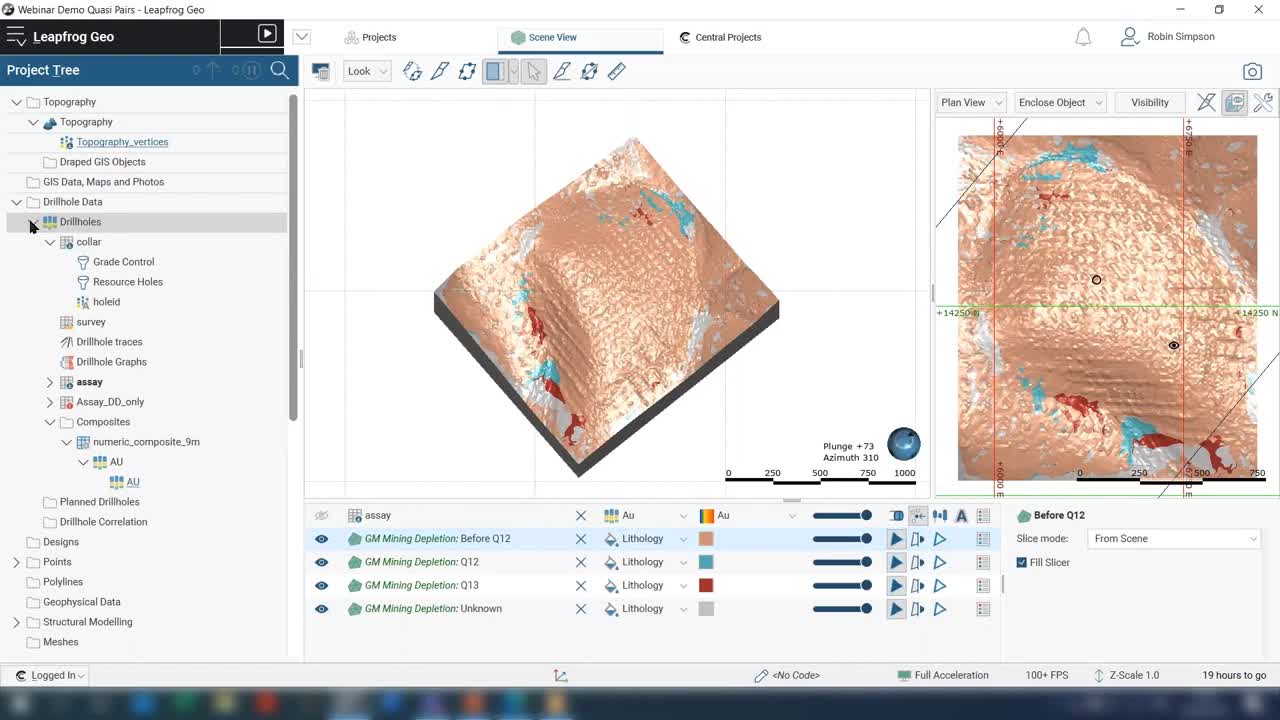
Now, the dataset I’m using,

[00:04:36.700]
the client’s asked me not to reveal the name of the deposit,

[00:04:39.830]
so I’ve decided it’s open pit gold deposit.

[00:04:43.020]
It’s a mixture of core drilling and blast hole samples.

[00:04:47.210]
And we have some mining topography surfaces

[00:04:50.890]
that represent the pit position at the end of each quarter.

[00:04:54.990]
So based on these topography surfaces,

[00:04:58.670]
the geological model I’ll be using is actually

[00:05:01.300]
a model of the different increments of depletion.

[00:05:04.660]
So we can look at the blast hole samples

[00:05:08.598]
through different time increments.

[00:05:12.867]
So I’m focusing here on an example that’s

[00:05:15.920]
blast hole data versus core data,

[00:05:19.220]
which is a very common problem,

[00:05:21.780]
or a very common aspect you need to analyze

[00:05:25.040]
when reviewing gold deposits.

[00:05:27.210]
But the same technique, I think you will see,

[00:05:31.270]
could be applied to diamond core versus RC,

[00:05:35.918]
or to drilling versus channel sampling,

[00:05:38.040]
different campaigns of drilling

[00:05:40.850]
or to actual twin holes where perhaps the twin holes

[00:05:45.030]
have been colored on different elevations

[00:05:47.920]
and you’re looking for a way to match those twins in space.

[00:05:55.650]
The statistical technique I’ll come back to

[00:05:59.830]
is the QQ Plots function in Leapfrog,

[00:06:02.880]
but I’ll talk more about what a QQ Plot actually is

[00:06:06.970]
when we get to that stage.

[00:06:08.480]
So go into the Leapfrog project now.

[00:06:11.300]
There’s the starting point, assuming that you’ve got

[00:06:14.620]
your drill hole database already set up.

[00:06:19.720]
And you’ve got some sort of filter on the color table

[00:06:23.090]
that will allow you to split the different data types

[00:06:26.810]
or different campaigns.

[00:06:29.370]
So, showing you this database here.

[00:06:35.480]
Which you can see, there’s a lot of blast holes,

[00:06:40.910]
tens of thousands or maybe even hundreds of thousands.

[00:06:43.910]
And then you’ve got the,

[00:06:47.460]
the resource holes

[00:06:49.560]
on a fairly regular grid,

[00:06:52.260]
but with some areas with closer spacing.

[00:06:58.550]
On the color table, we’ve got filters set up

[00:07:03.079]
that split the database into two types,

[00:07:09.010]
the gray control holes, the blast holes,

[00:07:12.990]
and the resource holes,

[00:07:15.060]
which are mostly diamond holes with a few RC.

[00:07:22.549]
The other thing I’m assuming that’s already been set up

[00:07:25.610]
is whatever geological model you want to use

[00:07:29.310]
for dividing up the analysis.

[00:07:31.890]
Potentially you can do this type of analysis

[00:07:33.810]
completely unconstrained,

[00:07:36.586]
that may be useful at the very early stage.

[00:07:41.205]
Just about always though,

[00:07:42.600]
statistical analysis is improved

[00:07:44.457]
if you are constrained by some simple domain.

[00:07:50.420]
As I said, the geological model in this case

[00:07:53.073]
that we’re using to split the analysis

[00:07:55.310]
is not really geology at all.

[00:07:56.303]
It’s a series of depletion topographies,

[00:08:01.240]
so in particular we’re going to look at

[00:08:04.500]
well that’s showing how all the depletion so far looks.

[00:08:09.220]
And then within that we’ve got volumes

[00:08:13.520]
representing different increments of depletion.

[00:08:21.430]
Now the first step,

[00:08:22.990]
assuming that database geological model are in place,

[00:08:26.340]
is to decide on the appropriate compassing width

[00:08:29.870]
comparison.

[00:08:32.760]
It may be useful to go to the

[00:08:34.880]
essay element of your drill hole database

[00:08:39.180]
and statistics.

[00:08:42.500]
Sorry, I’m not on, not on the actual gold value itself

[00:08:44.800]
for the statistics on the main file,

[00:08:47.200]
the interval link statistics.

[00:08:52.230]
And that will show you a histogram of,

[00:08:57.850]
multiple links and you can potentially filter that

[00:09:00.440]
just by one of the data types.

[00:09:04.690]
So for these, these blast hole samples,

[00:09:08.010]
you can see that there’s really two,

[00:09:10.350]
two peaks in the distribution,

[00:09:11.810]
one at six meters and one at nine meters

[00:09:14.340]
and perhaps a smaller peak at about 12 meters.

[00:09:18.380]
Now, I know from looking at this earlier,

[00:09:20.620]
that in the area that I’m really interested in,

[00:09:24.070]
it’s almost entirely nine meters.

[00:09:26.328]
So there’s that peak there applies.

[00:09:30.280]
So, the composite length we’ll use for,

[00:09:33.130]
for the comparison is going to be mid nine meters.

[00:09:39.280]
But the idea is we’re going to standardize the,

[00:09:41.157]
the blast holes, which are generally on nine meters

[00:09:44.750]
with the resource holes,

[00:09:47.310]
which are obviously sampled in something smaller,

[00:09:50.130]
but to equalize the support

[00:09:52.250]
or approximately equalize the support,

[00:09:55.230]
we will composite the diamond hole to nine meters.

[00:10:01.160]
So the next step is to, in the composites folder,

[00:10:04.920]
a new numeric composite,

[00:10:08.109]
and it’s a simple entire drill hole

[00:10:11.330]
without any domain applied.

[00:10:15.850]
Choose nine meters as the length,

[00:10:18.760]
but then whatever rules

[00:10:20.430]
you might think will be appropriate for residuals.

[00:10:24.040]
Oh, just make something up for now.

[00:10:35.110]
And it’s just the gold value from the essay table.

[00:10:39.950]
I know now compositing in the drill hole database here

[00:10:42.600]
doesn’t give you the option of any filter,

[00:10:44.550]
so it’s going to even composite everything,

[00:10:48.880]
including the blast holes to nine meters.

[00:10:51.710]
And given that there’s I think

[00:10:53.340]
hundreds of thousands of blast holes there,

[00:10:55.930]
When we run this,

[00:10:57.610]
it can take quite a bit of processing time

[00:10:59.990]
to do a nine meter composite of the entire database.

[00:11:03.780]
If your database is a

[00:11:05.260]
mixture of both ground control and resource,

[00:11:08.880]
there are workarounds to speed that up.

[00:11:12.620]
For now I’ll just say let’s, let’s wait it out.

[00:11:15.618]
Or I’ll take a shortcut and tell you

[00:11:18.080]
that I’ve already prepared the composites earlier.

[00:11:20.340]
So you don’t have to

[00:11:22.210]
spend 20 minutes waiting for me to process that.

[00:11:27.898]
So it’s assuming we’ve generated those composites

[00:11:32.210]
then from that composites of everything in the database,

[00:11:37.700]
one way to just get the resource whole composites,

[00:11:44.680]
which is what we’re going to use

[00:11:46.970]
as part of our pairing analysis

[00:11:49.600]
is to go to the points folder.

[00:11:53.230]
New interval mid points,

[00:11:56.170]
and then we select our nine meter composites,

[00:11:58.880]
and then we put on that filter that just selects the

[00:12:03.450]
resource holes.

[00:12:08.820]
The alternative would be to, you can,

[00:12:10.610]
at this stage use the blast holes,

[00:12:13.250]
or just select the blast holes.

[00:12:16.090]
I would recommend in terms of processing time

[00:12:18.550]
for the workflow I’m demonstrating here.

[00:12:21.160]
You, you choose the composites that are the smaller group

[00:12:26.450]
or the one with a fewer composites.

[00:12:30.120]
So which in this case is the resource holes.

[00:12:45.910]
So I’ve, that’s quite quick to process

[00:12:49.240]
and I’ve generated this points file from the mid points

[00:12:51.960]
of just the diamond holes.

[00:12:59.120]
Now onto that file while we’re here,

[00:13:03.970]
evaluations

[00:13:06.390]
and whatever geological model you might be using

[00:13:11.330]
to divide your analysis,

[00:13:14.370]
you evaluate that onto this point’s file.

[00:13:16.980]
So in this case, it’s a mining depletion model.

[00:13:25.900]
The other preparatory step you can do at this stage

[00:13:29.300]
is to create a capped value.

[00:13:32.720]
So that’s under calculations and filters.

[00:13:39.750]
Numeric calculation,

[00:13:44.524]
I’m going to tap it at four.

[00:13:48.715]
And then it’s, when you’re creating a text like this

[00:13:52.277]
,by using an if statement.

[00:13:57.260]
So if you aspire to in four that’s four

[00:14:02.250]
otherwise,

[00:14:06.100]
it’s just a year

[00:14:10.030]
and save that.

[00:14:15.360]
So that’s prepared our points file with the,

[00:14:19.770]
the resource or the mostly diamond composites.

[00:14:24.520]
Now the other part of the pairing,

[00:14:25.880]
we will now go to estimation

[00:14:29.200]
and we’ll work with the blast holes.

[00:14:39.230]
So select domain, this is where you can

[00:14:44.780]
choose one of the domains from your geological model.

[00:14:51.000]
It’s that one, or if you wanted to do unconstrained pairing,

[00:14:55.177]
you can just choose the boundary.

[00:14:56.950]
There is a shortcut to

[00:15:00.070]
a meeting the requirement for having

[00:15:01.590]
something in the domain, but, but effectively,

[00:15:04.780]
including the entire volume of your model

[00:15:07.980]
when the trial volume of the deposit.

[00:15:11.650]
Choose that that option there,

[00:15:16.950]
and the inputs will be,

[00:15:18.550]
are you from the sample table

[00:15:21.350]
with the pride control filter on,

[00:15:26.088]
I’m going to say no compositing newer,

[00:15:28.730]
because freight control samples

[00:15:30.680]
are already on a fairly standard length.

[00:15:46.205]
So, we’ve created a new estimation,

[00:15:48.660]
and then in that estimation, down estimators,

[00:15:54.450]
new nearest neighbor estimator,

[00:15:57.960]
and this might have to wait for the processing to happen.

[00:16:06.410]
All right, well, I’ll go to the ones I prepared earlier.

[00:16:08.330]
So we don’t have to wait for that

[00:16:10.367]
and show you how it’s done.

[00:16:20.773]
Here is estimators,

[00:16:23.680]
new nearest neighbor estimator

[00:16:27.070]
value clipping.

[00:16:28.010]
So this is where we can put on some capping.

[00:16:33.040]
It’s the same capping we put on the diamond composites

[00:16:37.670]
and where it says ellipsoid.

[00:16:40.810]
This is where you are effectively choosing

[00:16:43.470]
a maximum pairing distance for creating these paired,

[00:16:47.051]
these paired composites.

[00:16:49.660]
So you use quite a tight search ellipsoid.

[00:16:54.890]
And in this case,

[00:16:55.723]
it might get a simple sphere with radius tin.

[00:16:59.230]
So this means that for the pairing

[00:17:02.910]
where we’re going to be creating peers

[00:17:04.890]
that are no more than 10 meters apart in any direction.

[00:17:14.030]
And that’s all we need to specify there.

[00:17:25.010]
And once you’ve created that estimator,

[00:17:28.230]
then you go back to the points file

[00:17:31.630]
with the diamond composites

[00:17:36.893]
and you evaluate that estimator

[00:17:46.200]
onto the points.

[00:17:52.980]
That evaluation should be quite quick.

[00:18:03.880]
So now with, on that points file, we have

[00:18:09.590]
both the information from the diamond composites

[00:18:13.780]
and the original points, and we got,

[00:18:15.750]
got the peered values from the blast soul samples

[00:18:21.580]
for via this evaluation.

[00:18:24.080]
There are a couple more filters we need to set up

[00:18:28.076]
before we can get to the analysis.

[00:18:31.460]
So,

[00:18:35.480]
I’ll show you the stats on the slope work.

[00:18:41.100]
If you, if you look at the statistics for the evaluation,

[00:18:46.010]
you will notice there are a lot of negative one values

[00:18:49.510]
in there.

[00:18:50.800]
This cause LeapFrog’s inserting negative one,

[00:18:54.380]
where it’s not finding a,

[00:18:58.550]
a blast hole sample

[00:19:00.170]
within that 10 meter search range

[00:19:02.300]
of the diamond composite and midpoint.

[00:19:06.610]
So for further evaluation, further analysis,

[00:19:09.150]
we want to exclude those negative ones.

[00:19:12.940]
And we also probably want to set up a filter,

[00:19:16.480]
that’s going to divide it

[00:19:18.440]
according to the domains from a geological model.

[00:19:24.960]
So tidy this up and close a few windows.

[00:19:34.940]
Back to calculations and filters.

[00:19:38.990]
New filter,

[00:19:42.019]
and we’ll call this

[00:19:45.767]
“Pairs

[00:19:47.620]
and the

[00:19:53.590]
quarter 12 domain”

[00:19:58.480]
Really two parts to this filter.

[00:20:01.330]
So in the mining depletion

[00:20:02.830]
from the Von mining depletion evaluation,

[00:20:05.330]
it’s that equals

[00:20:08.710]
before quarter 12.

[00:20:11.623]
And the other part is

[00:20:14.550]
the nearest neighbor evaluation

[00:20:20.130]
must be greater zero.

[00:20:27.940]
So let’s sit up now.

[00:20:31.690]
We’ll see how those

[00:20:34.840]
points look in 3D.

[00:20:39.660]
So the,

[00:20:43.760]
here are the, all the

[00:20:48.180]
diamond composites in her file,

[00:20:50.130]
kept at four,

[00:20:55.480]
we can filter it.

[00:20:57.663]
So it’s just

[00:21:00.810]
the pairs that are in that particular

[00:21:05.060]
lump of depletion

[00:21:13.890]
and have blast holes

[00:21:16.890]
within

[00:21:18.280]
10 meters.

[00:21:22.130]
Check that, so that’s the nearest neighbor evaluation.

[00:21:30.030]
That’s what it looks like in 3D.

[00:21:32.640]
And then we can start making statistical comparisons.

[00:21:35.500]
And the, the simplest is just to look

[00:21:37.470]
at the uni variant stats.

[00:21:40.380]
So on our

[00:21:43.132]
kept diamond composites,

[00:21:47.910]
we have

[00:21:50.270]
5,937 composites

[00:21:53.690]
that meet that condition of being

[00:21:55.060]
within that particular zone of depletion

[00:21:57.540]
and paired with a,

[00:21:59.950]
a blast hole grade.

[00:22:04.510]
So the mean value of those is about 0.6.

[00:22:09.380]
And similarly,

[00:22:10.213]
we can look at these statistics for the period values.

[00:22:19.090]
So the main value is about 0.61.

[00:22:20.890]
So there’s,

[00:22:21.723]
there’s not much difference in mean

[00:22:24.150]
just from those quick comparison

[00:22:26.410]
of histograms and summary statistics,

[00:22:32.520]
but a more, more informative comparison is,

[00:22:38.570]
is the QG plot.

[00:22:42.490]
For those of you who may not be familiar with this tool,

[00:22:45.400]
I’ll, I’ll explain briefly

[00:22:49.410]
how it works.

[00:22:52.560]
So, a QQ plot

[00:22:56.540]
can be used wherever you have two sets of data.

[00:23:00.430]
The two sets of doubt don’t have to be of the same size.

[00:23:03.710]
Now, in the case, we’re using it here.

[00:23:05.270]
They are of the same size because of they’re pairs,

[00:23:08.760]
but QQ plot doesn’t rely on that pairing link.

[00:23:16.340]
Then once you have the two sets of data,

[00:23:20.220]
then you calculate quantiles,

[00:23:23.610]
which happens by ranking each to data set in order

[00:23:28.820]
and then picking you out numbers

[00:23:32.060]
at certain points in the ranking

[00:23:34.840]
that correspond to quantiles.

[00:23:38.080]
Now usually the quantiles are talking about a percentiles

[00:23:41.510]
in this very quick, rough example shown here

[00:23:44.400]
I’m using deciles.

[00:23:45.940]
So, so every, points are at 10% increments of the data.

[00:23:52.580]
So this, how I see it has 10 values.

[00:23:55.020]
This has 20 values.

[00:23:57.810]
So when we do our quantiles, we’re using all of those.

[00:24:02.850]
And when we’re using the quantile or the decile

[00:24:05.570]
or somebody said for 20 values for using every second value.

[00:24:10.230]
So after ranking and

[00:24:13.830]
doing these selection based on the certain percentages,

[00:24:18.090]
then we plot the quantiles against each other.

[00:24:21.560]
And that’s,

[00:24:23.010]
that’s what gives us a chart that looks like this.

[00:24:25.000]
Now, normally we’re dealing with much larger data sets,

[00:24:30.050]
but this simple example shows,

[00:24:32.280]
shows the mechanics of what’s going on.

[00:24:36.320]
So I go back to the LeapFrog project.

[00:24:38.930]
Now this happens and LeapFrog.

[00:24:41.340]
So you would click on

[00:24:45.600]
Statistics

[00:24:46.780]
Right click on the file, the points file statistics,

[00:24:49.650]
QQ plot,

[00:24:52.800]
the X input will say the,

[00:24:56.890]
the kept grades from the diamond composites.

[00:25:02.290]
We put on that filter restricted

[00:25:05.370]
to the certain name we’re interested in

[00:25:09.640]
the wides, the nearest neighbor evaluation.

[00:25:12.540]
Again, with the filter,

[00:25:15.490]
and we get a chart that looks like this,

[00:25:17.660]
and you can put it on the one-to-one line

[00:25:21.670]
for information as well.

[00:25:24.640]
So, so in that case, that example,

[00:25:26.310]
there is showing that there is actually a,

[00:25:30.170]
quite a good relationship between the blast hole samples

[00:25:33.787]
and the diamond core samples.

[00:25:38.870]
If you’ve done as a simple scatter plot,

[00:25:41.590]
which we can also do,

[00:25:45.720]
and using the same sort of inputs,

[00:25:57.100]
you get a bit of a mess, and it might be difficult to read,

[00:26:00.060]
anything matched into that, but with the QQ plot

[00:26:03.779]
and the way it’s ordering and ranking by percentiles,

[00:26:08.261]
it shows that the distribution of

[00:26:12.580]
diamond composites within this domain

[00:26:15.400]
is very similar to the distribution of blast holes,

[00:26:20.440]
which can actually be a surprising result.

[00:26:22.200]
If you’ve seen blast hole sampling done in practice,

[00:26:25.060]
it often looks awful

[00:26:28.438]
and many cases,

[00:26:30.910]
You wonder how you can possibly get a representative sample

[00:26:33.180]
from it, but for this deposit,

[00:26:35.490]
it seems actually to be working quite well.

[00:26:42.880]
That was just one of those depletion increments.

[00:26:47.930]
In this case, I’ll use the file I prepared earlier.

[00:26:52.250]
I’ll show you what it looks like when preps, the,

[00:26:54.520]
the two sets of data don’t match up so well

[00:26:58.220]
for this quarter 12.

[00:27:11.170]
Now show the quarter 13. Okay. So.

[00:27:14.450]
If you look at that QQ plot,

[00:27:16.870]
you can see that

[00:27:20.150]
the low values and the high values of the distributions

[00:27:22.950]
match up reasonably well.

[00:27:25.690]
But in between, it seems as though the,

[00:27:32.770]
the curve is dropping below the one-to-one line,

[00:27:34.950]
which in this case means that the,

[00:27:39.060]
the diamond information diamond core information is

[00:27:44.220]
biased higher relative to the blast hole.

[00:27:47.440]
Self-incrimination

[00:27:51.160]
that was quarter 13,

[00:27:54.420]
quarter 12.

[00:28:04.723]
Yeah.

[00:28:15.179]
so the diamond composite information is on the X

[00:28:20.310]
Blast holes on the Y.

[00:28:22.530]
This is showing you an example where

[00:28:25.130]
you have a things reasonably good up to about 1.3, 1.4.

[00:28:31.030]
And then we start to see the blast holes

[00:28:34.200]
being somewhat biased high relative to the diamond core.

[00:28:40.690]
So those are reasonably real examples of what

[00:28:46.113]
QQ plots can look like.

[00:28:50.450]
And the QQ plots revealing a bit more than,

[00:28:52.950]
than just the, the univariate sort of sets,

[00:28:56.814]
or looking at the means of the two sets about it would.

[00:29:01.280]
So that’s, that’s the workflow up to using QQ plots.

[00:29:06.600]
There would be other types of analysis you can do,

[00:29:10.986]
or just do a summary of what’s happened.

[00:29:18.660]
Okay, so the workflow that’s mentioned

[00:29:20.430]
before starting you seem that you had the database set up

[00:29:23.650]
geological model set up,

[00:29:25.390]
and you had filters on the Color table

[00:29:26.970]
that divide your data into different types.

[00:29:31.530]
And you choose the composite length you’re going to use for

[00:29:33.940]
the analysis.

[00:29:36.507]
In this particular case, the influenced statistics tool

[00:29:40.457]
on the essay table can be useful.

[00:29:45.560]
And the composites folder of your database

[00:29:49.020]
make numeric composites at that length.

[00:29:53.200]
And then the way we split out a one,

[00:29:57.060]
one data type from those composites

[00:29:58.790]
is to use the interval midpoints option

[00:30:01.610]
in the points folder.

[00:30:04.270]
And at that stage, I recommend choosing as your valor type,

[00:30:08.650]
this first stage is one of the fewer holes.

[00:30:14.350]
Evaluate the geological model onto those points.

[00:30:17.850]
Potentially set up a capping grade on those points,

[00:30:23.420]
and then go to the estimation folder

[00:30:25.340]
and set up a new domain destination

[00:30:28.330]
where the input will be any domain

[00:30:31.020]
you want to use to constrain,

[00:30:33.623]
and you filter be the composites of samples five,

[00:30:37.220]
whatever the second data type is

[00:30:41.890]
within the estimation credit, nearest neighbor estimator

[00:30:45.230]
with a reasonably tight search distance

[00:30:48.130]
and set a capping on that estimator.

[00:30:51.780]
And then you evaluate that nearest neighbor estimator

[00:30:55.010]
onto the midpoints that contain the,

[00:30:57.560]
the first part of pairing

[00:31:01.970]
with that file with the,

[00:31:04.960]
the paired points and the paired points

[00:31:07.140]
for the nearest neighbor evaluation.

[00:31:09.320]
Set up filters to split by domain

[00:31:12.410]
and to exclude

[00:31:14.646]
anywhere where there’s been a default negative one assigned,

[00:31:17.800]
which will mess up your statistics.

[00:31:21.440]
Once you’ve done all that,

[00:31:22.500]
then you can go and start analyzing the pairs

[00:31:26.380]
with either various statistics

[00:31:29.040]
or the QQ plot can be quite useful.

[00:31:33.820]
So headed back to Carrie for any questions.

[00:31:38.210]
<v Carrie>Thank you, Robin.</v>

[00:31:39.060]
Thank you for your presentation.

[00:31:42.910]
Robin is available to take questions.

[00:31:45.210]
So if you have any questions,

[00:31:47.100]
please type them in the questions box,

[00:31:51.036]
and then we can.

[00:31:54.248]
Give it to Robin to answer them.

[00:31:57.709]
I, I don’t see any questions in the box at the moment,

[00:32:03.130]
but Robin, I’ll ask you a couple of my own here.

[00:32:07.670]
So for similar examples to the case study,

[00:32:10.580]
what are some approaches that could be used

[00:32:13.030]
if the grade control and resource drilling data,

[00:32:15.250]
not already combined into one database?

[00:32:21.224]
<v Robin>You know, well Carrie the,</v>

[00:32:22.817]
if they are in one database,

[00:32:25.440]
sometimes it can actually cause a problem

[00:32:27.770]
because of the, the compositing of everything.

[00:32:30.921]
So, it can be very slow.

[00:32:32.290]
And if it has to churn through

[00:32:34.600]
hundreds of thousands of blast hole samples.

[00:32:38.820]
So, if your database just has the reasonable samples,

[00:32:43.210]
it may be possible to import the blast hole samples,

[00:32:47.620]
from another database, just as X, Y, Z points.

[00:32:51.630]
Not as input tables,

[00:32:53.307]
and if those blast holes are already standard lengths,

[00:32:57.250]
you don’t need to do anymore depositing

[00:32:58.780]
so, just importing the midpoints

[00:32:59.913]
through the holes will be sufficient.

[00:33:03.310]
Another thing is that with the latest version of LeapFrog

[00:33:08.140]
I see there’s an option for a lot more databases.

[00:33:12.430]
I haven’t used this much myself yet,

[00:33:14.550]
but this may also make it, the process work better

[00:33:18.100]
because if you have the blast holes in a separate database

[00:33:21.639]
then when you do the general depositing

[00:33:23.540]
on the resource holes,

[00:33:26.020]
that depositing doesn’t need to run

[00:33:27.620]
through blast holes as well.

[00:33:31.870]
<v Carrie>Sure, great. Thank you. Thanks for that</v>

[00:33:35.620]
We do have a question,

[00:33:38.030]
from one of the attendees now, from Evan

[00:33:42.170]
He asked, “Did you make the nearest neighbor estimation

[00:33:45.430]
on all data or only on the blast holes?”

[00:33:51.490]
<v Robin>Yeah so the way I set up,</v>

[00:33:53.274]
the nearest neighbor estimation was

[00:33:55.440]
the blast holes is the inputs

[00:33:58.150]
and then evaluate that onto the diamond composite

[00:34:01.850]
as the output.

[00:34:05.590]
It will be possible to do it in reverse as well.

[00:34:08.220]
To do a similar analysis, with using the resource

[00:34:11.210]
as the input and the blast holes as the output.

[00:34:14.230]
I often stand to practice, that it runs a bit faster

[00:34:18.990]
if you choose the,

[00:34:21.180]
the input

[00:34:23.720]
for the nearest input

[00:34:25.940]
the more circles in it.

[00:34:28.210]
So I hope that answers the question.

[00:34:32.340]
It didn’t run it’s nearest neighbor

[00:34:35.470]
on everything all at once.

[00:34:36.910]
We did separate

[00:34:39.440]
the diamonds and blast holes

[00:34:42.440]
based on the filters we did on the color table.

[00:34:49.070]
<v Carrie>Great, thank you.</v>

[00:34:50.120]
So Evan, I hope that answers your question.

[00:34:55.100]
Oh, I’ll ask you another one from myself here.

[00:34:58.140]
So in the case study, 9 meter composite length was used

[00:35:01.727]
assessing of the QQ plot comparison,

[00:35:05.560]
so does this choosing of the relatively long length

[00:35:08.220]
for the diamond drilling composites,

[00:35:09.670]
have any barring of the composite length

[00:35:11.510]
that would then actually be used for

[00:35:13.550]
setting up the rigging estimate.

[00:35:17.750]
<v Robin>Oh, it doesn’t need to, I mean</v>

[00:35:19.660]
the 9 meter length was necessary to make the support

[00:35:24.427]
to the break control information for this analysis.

[00:35:29.340]
9 meters is certainly a long length.

[00:35:31.400]
It would be what most people would use

[00:35:34.898]
for resource estimation diamond,

[00:35:36.150]
or one or two meter diamond ore.

[00:35:38.427]
Like diamond samples.

[00:35:40.920]
But once you’ve done this assessment

[00:35:43.280]
and decided whether or not there’s any bias.

[00:35:46.239]
They can be entirely separate with how you proceed

[00:35:49.170]
with the reasonable estimation, using only the blast hole.

[00:35:52.871]
Without using the resource holes.

[00:35:57.108]
And you’d probably revert to it.

[00:35:59.650]
Probably, a one or two meter composite length for that.

[00:36:04.460]
<v Carrie>Yeah, sure I think, yeah, some good advice there.</v>

[00:36:12.540]
Last question from me.

[00:36:14.250]
So don’t see any more questions in the question box.

[00:36:16.930]
So in the case study, you did the analysis by domain.

[00:36:21.340]
Is this always necessary,

[00:36:23.570]
or could you do on the deposit scale?

[00:36:25.220]
what would be your thought process on deciding, you know,

[00:36:29.090]
to what scale you would do the study on?

[00:36:32.863]
<v Robin>It depends on how,</v>

[00:36:34.870]
how much information available

[00:36:36.680]
and whether your domains are prepared yet.

[00:36:39.050]
Or you can go ahead with this analysis

[00:36:42.020]
even before you’ve prepared any domains

[00:36:44.070]
and just do it as unconstrained,

[00:36:46.270]
and then repeat it as you develop and test your domains,

[00:36:50.970]
somewhat constrained by you need probably

[00:36:53.960]
several hundred pairs to get a useful QQ plot.

[00:36:59.320]
So,

[00:37:00.247]
which domains you use

[00:37:03.380]
and what level of detail and remaining

[00:37:06.430]
you apply to this that does depend on that constraint of

[00:37:10.060]
making sure you actually capture enough pairs

[00:37:12.520]
to make it worthwhile

[00:37:14.250]
that the pairing can be adjusted by,

[00:37:18.300]
by playing with the, the search distance.

[00:37:21.670]
I use 10 meters that example,

[00:37:24.320]
and you might move that up or down by a few meters,

[00:37:29.628]
so that the process isn’t dependent on domains,

[00:37:33.860]
but like most statistical analysis

[00:37:37.650]
things are improved by

[00:37:39.390]
using domains as much as possible.

[00:37:42.480]
<v Carrie>Yeah, sure. Yeah. Yeah. I guess, yeah.</v>

[00:37:44.700]
It’s depending on the amount of data.

[00:37:46.960]
Great. Thank you.

[00:37:48.770]
We had a question come in from Laura.

[00:37:52.410]
She asked, “Is this method to create the twin pairs

[00:37:55.650]
still efficient with another estimator,

[00:37:58.030]
such as Coke rigging.

[00:38:05.460]
<v Robin>At this stage, I’m just,</v>

[00:38:07.273]
just doing it as a very simple pairing exercise, not,

[00:38:10.840]
not trying to bring any vary grams or,

[00:38:13.690]
or weighted estimates in.

[00:38:16.540]
Sense of using

[00:38:18.459]
the nearest neighbor,

[00:38:21.305]
just as a method of making pairs.

[00:38:23.613]
It’s not really as a, as an estimator itself,

[00:38:27.890]
if going to bring in techniques like Coke rigging.

[00:38:32.580]
Now that implies that you’ve already done some details,

[00:38:36.270]
statistical analysis and interpreted

[00:38:39.350]
variant vary grams across vary grams,

[00:38:42.250]
Whereas, I’m seeing this method had been more useful earlier

[00:38:46.510]
in the analysis process.

[00:38:49.790]
<v Carrie>Okay. All right.</v>

[00:38:52.200]
Hopefully that answers your question. Laura,

[00:38:55.970]
has anyone got any other questions?

[00:38:58.480]
I don’t have any from my side,

[00:39:00.160]
so there’s no more questions we’ll, we’ll finish up.

[00:39:07.970]
So I don’t think there’s anything more coming through here.

[00:39:11.920]
So just lastly then to, to round off,

[00:39:14.510]
thank you for attending today.

[00:39:16.760]
And I hope that, you know,

[00:39:18.390]
you find this will find this,

[00:39:20.200]
a useful technique that you will try in the future.

[00:39:23.370]
If you want to get in touch with anyone here at Seequent or

[00:39:26.970]
with, if you want to contact Robin, SRK

[00:39:30.080]
Robin is on [email protected].

[00:39:36.090]
And at Seequent, you can support us, oh sorry,

[00:39:37.880]
contact us at [email protected]

[00:39:40.800]
for your technical queries or more kind of a licensing

[00:39:44.410]
and sales queries are at [email protected].

[00:39:49.190]
Okay, well, thanks very much, Robin.

[00:39:50.770]
Thank you as a great presentation

[00:39:52.790]
and thank you for answering the questions as well,

[00:39:56.250]
and I wish you all a good day.