


Leapfrog Works users can now access kriging for the first time with the new Contaminants extension. Existing Leapfrog users will be familiar with the Radial Basis Function (RBF) which is available in the Numeric Models folder. Now the RBF, Kriging, Nearest Neighbor and Inverse Distance estimators have been packaged together with a 3D variogram within the Contaminants extension, this allows users of the extension to compare results between different estimation methods.
All interpolation methods are designed to fill in the un-known spaces between known data in a way that can be mathematically and Geologically justified.
Kriging has historically been the preferred method for interpolation, however the RBF has relatively recently been widely adopted in the mining sector. Both methods are similar but with key differences. This article presents how the Leapfrog RBF, Ordinary Kriging and Simple Kriging relate to one another. We present methodology for matching kriging and RBF outputs with a real chlorinated plume data set.
Dataset
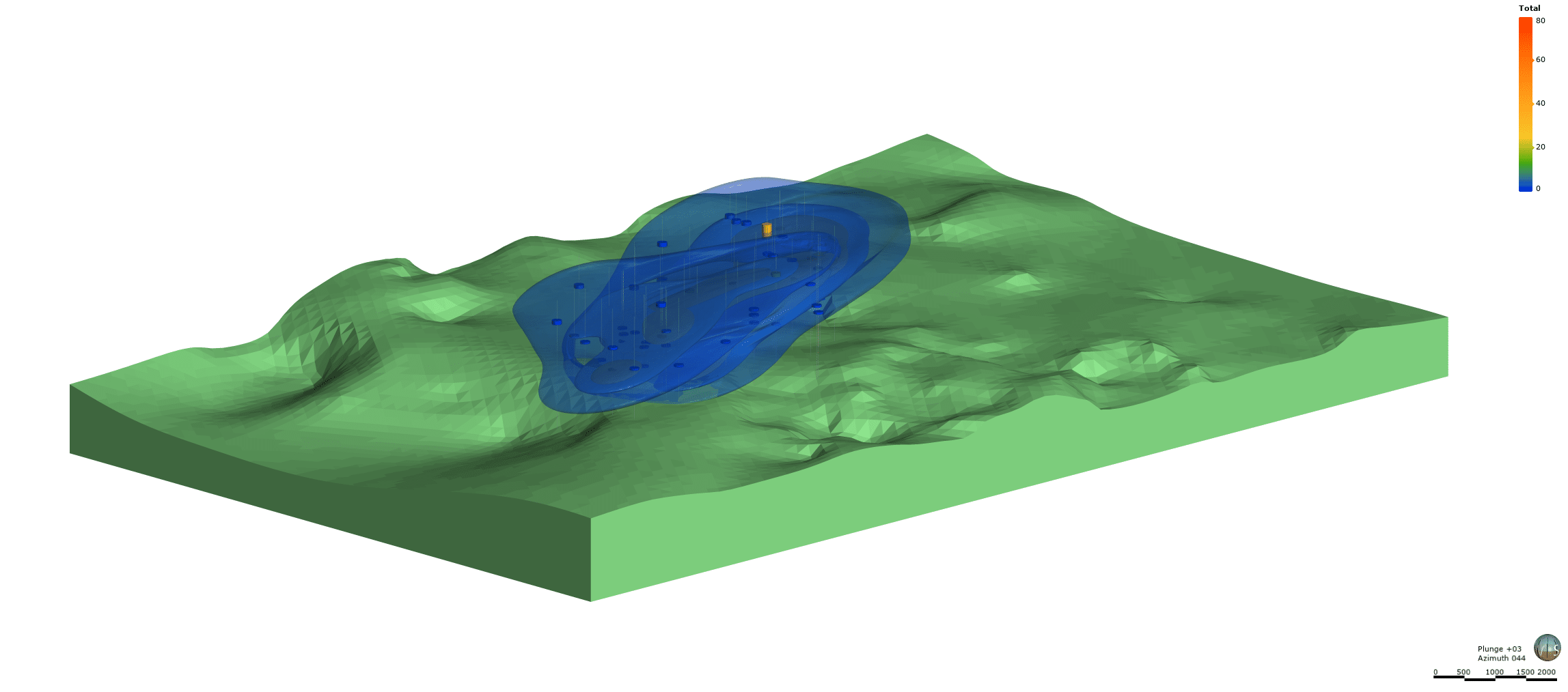
The data was acquired during 1993, from an area in the historically named Massachusetts Military Reservation main base landfill superfund site.
The dataset is comprised of ground water readings from 64 monitoring wells, which were drilled to monitor the extent of halogenated volatile organic compounds contained in the groundwater (Alden et al 1996). All the Contaminant data was log transformed prior to estimation.
What’s an RBF
Advances in software have enabled the implementation of radial basis functions (RBFs) as interpolation and extrapolation algorithms for both continuous (numerical) and categorical (geology) data. RBFs approximate a specific type of Kriging called Dual Kriging (Horowitz et al 1996), otherwise known as Global Kriging.
Like Kriging, RBF interpolation does not use an overly-simplified method for estimating unknown points, but produces a function that models the known data and can provide an estimate for any unknown point. Where Kriging is limited to a local search neighbourhood, RBF utilizes a global neighbourhood. Which makes the RBF ideally suited to producing continuous smooth plume models from sparse data.
What’s Kriging
Kriging involves two phases: variography (also an input for RBFs) and a process of Kriging. The variography indicates the distance after which it becomes useless to integrate data in order to determine the value we wish to find in a point, and the analysis of the variograms reveals the presence or the force of an anisotropic effect. This information, together with other constraints, allows us to choose the Kriging neighbourhood, i.e. the domain of the field that contains the site to be estimated and the data required to do so (Dauphiné et al 2017). The search neighbourhood is local but with Leapfrogs Kriging implementation it can be adjusted.
Ordinary and Simple Kriging only differ in the neighbourhoods the functions use and the value that they interpolate to, away from known data. Ordinary Kriging assumes a constant unknown mean over the search neighbourhood and the search neighbourhood can be constrained. Simple Kriging assumes stationarity of the first moment over the entire domain with a known mean. Both Kriging methods are available in the Contaminants extension.
Differences and similarities
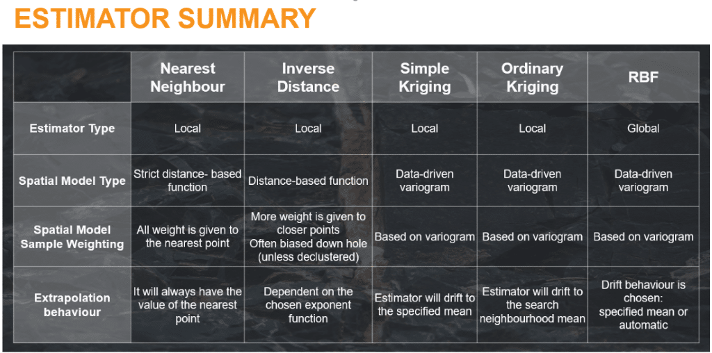
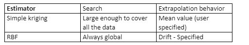
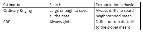
The key differences between Kriging and RBF estimators are how they are constrained and how they extrapolate away from known data. A summary of all the Contaminants extension estimators can be found in the table below.
Methodology for matching outputs
Leapfrogs Kriging implementation allows you to adjust the local neighbourhood by changing the search ellipsoid. Using a local or a global search depends on the type of problem you are trying to solve. A local search is useful for modelling the distribution of local values, where the data is highly variable. A global search is useful for modelling data with low variability, because the function will to a degree smooth the data across the entire domain.
A constrained local search will provide more accurate local estimates with highly variable data, but it can create undesirable interpolant artifacts, which a large search that incorporates all the data will not.
If the Kriging neighbourhood encompasses all the data, the interpolant extrapolation behavior is effectively global like an RBF. The other key difference is the type of drift, an Ordinary Kriging interpolant will drift to the search neighbourhood mean, Simple Kriging will drift to a user specified mean. The RBF has two drift settings. The drift can be automatic, which will also decay to the global mean (the mean of all the data in the domain) or it can be specified, where you can choose the value (a value greater than 0).
The RBF drift settings can be adjusted to match both Ordinary and Simple Kriging.
Comparison
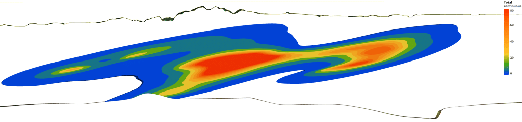
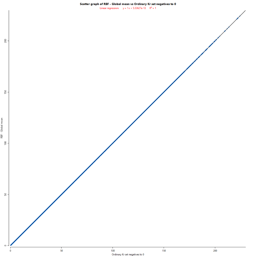
Swaths were taken through the middle of the plume to compare the difference between Ordinary Kriging, simple kriging with a mean of 0, RBF with a global mean drift and RBF with a user specified mean of 0.
Kriging Swath Plot

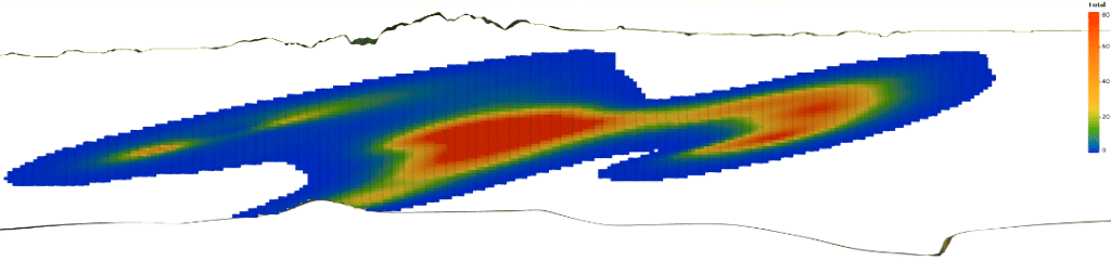
RBF Swath Plot
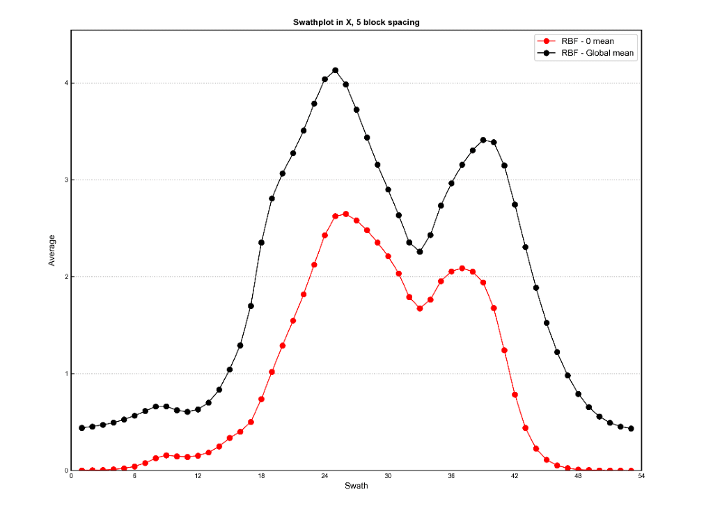
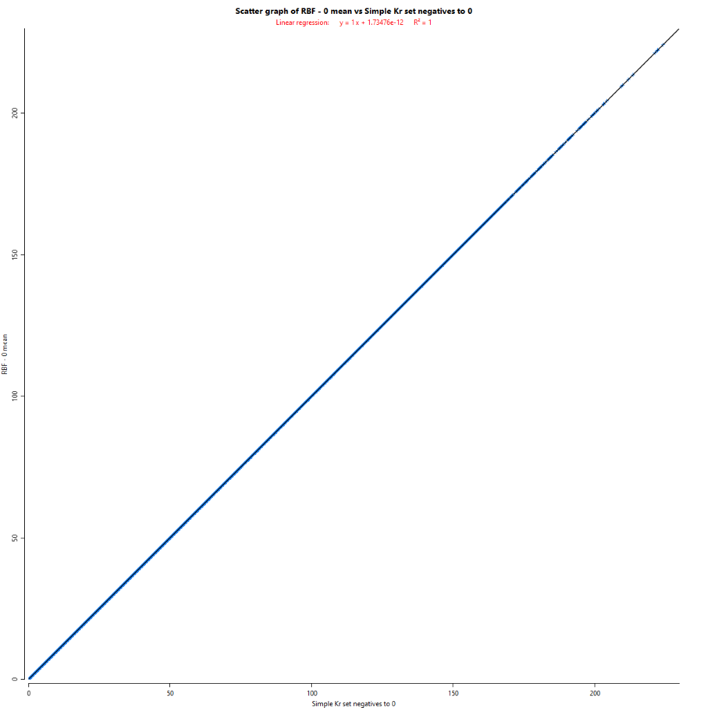
The Swath plot tool which is available in the contaminants extension, it’s a useful tool for comparing the results of different estimators, settings or variograms. For an alternative view of the correlation both combinations were plotted in scatter plots, each point represents a block model cell centroid.
Observations
- When the drift and search behavior is matched, both variations of Kriging and RBF estimator outputs are identical when assessed in swath plots and scatter plots.
- The drift setting makes a noticeable difference to the average Contaminant concentration.
- Matching RBF and Kriging outputs is dependent on increasing the Kriging search so that it covers all the data in the domain because Radial Basis Functions cannot have a local search.
- Interpolant methods are tools, the results are only as good as the input data and the assumptions applied by the user. The user still needs to apply sound Geologic knowledge and logic to interpolant model parameters.
Other resources
Theory of RBFs and Kriging and a comparison of estimates using a simulated gold data set.
Stewart M, de Lacey J, Hodkewicz P F and Lane R, 2014. Grade Estimation from Radial Basis Functions – How does it compare with Conventional Geostatistical Estimation? Proceedings of the Ninth International Mine Geology Conference (The AusIMM: Melbourne), pp. 129-142.
Arsenic concentration data set was interpolated using the ArcGis models: Inverse Distance Weighting (IDW), Ordinary Kriging (OK), and Radial Basis Function (RBF).
Carlos B. Manjarrez-Domínguez,1 Jesús A. Prieto-Amparán,2 M. Cecilia Valles-Aragón,1, M. Del Rosario Delgado-Caballero,3 M. Teresa Alarcón-Herrera,3 Myrna C. Nevarez-Rodríguez,1 Griselda Vázquez-Quintero,1 and Cesar A. Berzoza-Gaytan1. Arsenic Distribution Assessment in a Residential Area Polluted with Mining Residues. Int J Environ Res Public Health. 2019 Feb; 16(3): 375.
References
Horowitz F G, Hornby P, Bone D and Craig M, 1996. Fast Multidimensional Interpolations, Proceedings of the Application of Computers and Operations Research in the Mineral Industry (APCOM 26), Ramani R V (ed), (Society Mining Metallurgy and Exploration (SME): Littleton, Colorado), 583 p.
Alden D S, 1996. Subsurface Characterization of the Massachusetts Military Reservation Main Base Landfill Superfund Site.
Dauphiné A, 2017. Models of Basic Structures: Points and Fields. Geographical Models with Mathematica, Pages 163-197.