When Your Data Speaks Volumes

Overview

Video Transcript

[00:00:17.080]
<v ->Okay, hi there everyone.</v>

[00:00:19.210]
As Ryan just mentioned, my name is Sarah Conolly

[00:00:22.330]
and I’m part of the technical team

[00:00:24.070]
here in Vancouver for Seequent.

[00:00:26.812]
And today I’m going to be talking you though

[00:00:29.330]
my tips and tricks and they are called

[00:00:31.717]
“When your data speaks volumes”.

[00:00:34.380]
I gave it pretty vague title for this one.

[00:00:37.600]
If any of you know me from Geo,

[00:00:38.960]
that could mean pretty much anything in there.

[00:00:41.830]
But what we’re going to do today is

[00:00:45.200]
take a look a little bit further down

[00:00:47.470]
that mining value chain, so.

[00:00:50.750]
Jeff and Anna were, kind of earlier on,

[00:00:53.140]
Jeff found this bit for us, thanks Jeff.

[00:00:56.200]
Anna cleaned up my data,

[00:00:58.513]
and then I’ve actually got a model

[00:00:59.970]
that has been built in Leapfrog Geo.

[00:01:03.540]
I’m going to be moving closer towards my resource evaluation

[00:01:07.610]
and I’m actually going to be focusing on my EDA,

[00:01:10.280]
so my exploratory data analysis.

[00:01:13.750]
Hopefully to show you a few little tricks

[00:01:15.700]
using our interactive histograms to maybe think about how

[00:01:19.310]
you could further refine your geological model

[00:01:23.260]
and your estimation domains.

[00:01:24.850]
So I’m going to jump into Geo.

[00:01:42.010]
Excellent. Okay.

[00:01:43.760]
So, here we’re in the same deposit

[00:01:45.790]
that Anna and Jeff were looking at.

[00:01:47.630]
We’ve got two massive sulfide lenses here.

[00:01:50.780]
It’s a multi commodity deposit.

[00:01:53.640]
So we’ve got copper, zinc, lead, silver and gold.

[00:01:59.490]
My two massive sulfide lenses here

[00:02:01.700]
have been built from the geology.

[00:02:03.700]
So we’ve taken a look at our login information,

[00:02:06.060]
we’ve found those massive sulfide in stalls,

[00:02:07.890]
and we’ve created our volume.

[00:02:10.870]
I am going to look to one of those volumes

[00:02:14.840]
and just focus on this massive sulfide domain.

[00:02:17.810]
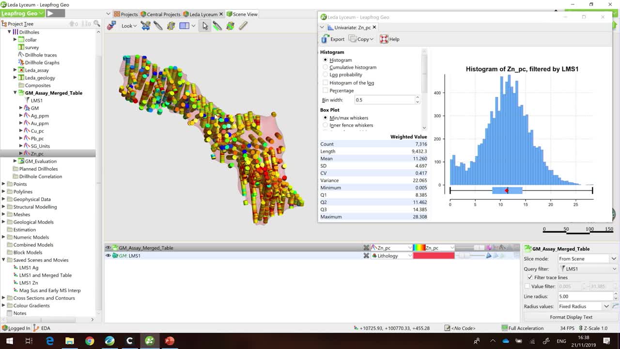
So here I’ve got that volume of interest.

[00:02:20.510]
I’ve got my data loaded and these,

[00:02:23.620]
I’m looking at my zinc assays.

[00:02:27.540]
But, I don’t understand the kind of statistics

[00:02:29.900]
that lie behind this and whether or not I’m happy

[00:02:31.977]
for my volume of interest to move forward

[00:02:34.430]
into my resource estimation.

[00:02:37.810]
So I’m going to take a look at a histogram of this data.

[00:02:43.470]
Just make this a little bit smaller,

[00:02:49.777]
so you can see them both. Okay.

[00:02:51.480]
So I’ve done a few things before we got here today.

[00:02:54.690]
I’ve merged my assay data with my geological information

[00:02:59.360]
and I’ve created a filter so I can sort them

[00:03:01.480]
looking at my values within this volume.

[00:03:04.635]
And I guess when I was first kind of started working

[00:03:10.460]
on grade control on models.

[00:03:12.740]
The first thing that I was taught

[00:03:14.140]
about my estimations of anything is that

[00:03:18.569]
you’ve got to have consistent geology.

[00:03:21.400]
I already told you that we have modeled this

[00:03:23.390]
from the login.

[00:03:25.040]
Obviously we validated that on like two photos

[00:03:29.505]
and I’m happy with that side of it.

[00:03:31.190]
Number two, that you’ve got one search orientation.

[00:03:35.380]
You could maybe argue that

[00:03:36.990]
there’s a little bit of folding in here,

[00:03:38.390]
but for today we’re going to go with, yep.

[00:03:40.280]
We’ve got that major twinge to our all body view.

[00:03:43.810]
Number three, that we have a single population

[00:03:47.100]
within that estimation domain.

[00:03:49.890]
And if you take a look at my histogram on the right here,

[00:03:52.870]
hopefully you can see we’ve got that

[00:03:54.330]
kind of classic bell curve that we’re after.

[00:03:56.620]
I’m fairly happy that I have one population.

[00:04:02.710]
Maybe take a look on the right hand side of my histogram.

[00:04:06.007]
You can see that around 25% of it

[00:04:09.458]
we’re actually getting a bit of a breakdown

[00:04:10.750]
in that population, and we’ve got a few outliers.

[00:04:15.420]
How do I find those outliers? And what do I do with them?

[00:04:19.370]
Do they cluster? Are they scattered?

[00:04:21.700]
Do I need to rethink my estimation domain?

[00:04:25.920]
Now I can build some filters to kind of try and find

[00:04:28.610]
where that data is.

[00:04:29.720]
However, in Leapfrog in the statistics tool,

[00:04:33.240]
all you need to do is click on your histogram

[00:04:37.230]
and those samples will appear in the scene.

[00:04:40.040]
So now, if I kind of spin around with my volume,

[00:04:43.620]
you can see those high grade outliers

[00:04:46.510]
are actually scattered through my domain.

[00:04:49.190]
And I’m probably more likely to deal with them with a

[00:04:52.230]
top cut or maybe some restrictions during my estimation.

[00:04:57.770]
So the zinc I’m pretty happy with to move forward.

[00:05:02.990]
If we take a little look at the silver distribution,

[00:05:08.090]
maybe we’ll see a different story.

[00:05:10.970]
And depending on what view you look at this, these assays.

[00:05:18.200]
The warm colors are representing the higher grade.

[00:05:20.810]
The cooler colors are a lower grade.

[00:05:23.700]
And hopefully you are seeing

[00:05:24.830]
that we have a fairly sharp contact

[00:05:28.720]
through the middle here.

[00:05:32.080]
But let’s have a look at the statistics behind this as well.

[00:05:34.820]
So I’m going to look at my silver histogram.

[00:05:39.210]
And unsurprisingly, it looks like we’ve got

[00:05:41.510]
a bi-modal distribution.

[00:05:43.120]
So instead of a perfect kind of bell curve

[00:05:45.780]
we’ve got a peak in the lower grades,

[00:05:48.770]
and then another peak in the second grades.

[00:05:52.610]
If we were to move forward with estimation

[00:05:54.610]
do these samples really relate to each other? Maybe not.

[00:05:58.440]
Maybe we’d want to sub domain this average

[00:06:00.760]
to separate units.

[00:06:02.830]
So again, these interactive histograms

[00:06:05.017]
can be really handy to do that.

[00:06:06.660]
So if I highlight the low grades, they gave me this scene.

[00:06:11.150]
If I highlight the high grades,

[00:06:13.950]
you get those intervals instead.

[00:06:16.980]
Which is great.

[00:06:19.270]
What’s the next step?

[00:06:20.900]
We want to split them out

[00:06:21.910]
and actually model them as separate units.

[00:06:24.670]
So if we layer up this interactive histogram,

[00:06:28.400]
with our interval selection tool.

[00:06:30.600]
We can then create a refined model

[00:06:32.480]
of our massive sulfide lens.

[00:06:34.610]
So I’m just going to create a new interval selection.

[00:06:39.040]
My silver domains.

[00:06:47.249]
And again, I’m just going to re highlight the low grade

[00:06:50.610]
samples and I’ll display them so you can see them.

[00:06:55.330]
And then I just use my select all visible intervals,

[00:06:59.240]
little button.

[00:07:00.950]
And I’m going to assign these to a new category.

[00:07:03.480]
So I’ll call this silver low grade.

[00:07:08.970]
Let’s go back to that interactive histogram.

[00:07:11.960]
Select the high grade.

[00:07:14.750]
Select all those little intervals.

[00:07:17.690]
And we’ll categorize these as our high grade.

[00:07:26.840]
So I’m done with my histogram now.

[00:07:29.260]
I’ll shut that down and save my interval selections.

[00:07:33.040]
And we can display them in the scene.

[00:07:36.440]
So now, rather than numeric data,

[00:07:38.430]
I’ve re-categorized that into my low grade samples

[00:07:41.830]
and my high grade samples.

[00:07:44.180]
And the next thing that I’m going to do

[00:07:46.250]
is actually use these to build another surface

[00:07:50.160]
in the middle of my volume of interest.

[00:07:52.920]
So if we go down to our geological models folder,

[00:07:57.480]
we can create what are called refined models.

[00:08:00.250]
And what they do, is that they’re basically going to take

[00:08:02.597]
the volume from the first pass model,

[00:08:05.020]
and then we can refine it like (undistinguishable)

[00:08:07.390]
I’m taking this massive sulfide lens

[00:08:11.031]
from my geology model.

[00:08:13.310]
I’m going to look to my new intervals

[00:08:20.640]
and create a new volume based off

[00:08:24.340]
the selections that I just created.

[00:08:27.330]
As I’m presenting I will create my volumes.

[00:08:31.860]
To my surfaces I’ll just hide those drill hole intervals.

[00:08:37.030]
So now we can see that within the volume of interest

[00:08:40.220]
I’m splitting it by those two different domains I created.

[00:08:44.490]
And as a final result,

[00:08:47.410]
I could move forward with the two separate volumes

[00:08:52.450]
on to my resource estimation.

[00:08:55.420]
So that was my little tips and tricks for today.

[00:08:58.265]
I was using my data to kind of build my confidence

[00:09:01.440]
in my output volumes to move on to estimation

[00:09:04.930]
at the end of the day.

[00:09:06.420]
Thanks for listening.

[00:09:07.776]
(crowd clapping)