VOXI: constrained modeling (Remote Roundup 2021)

Start with the basics, and build up to Geologically constrained model.

Overview

Video Transcript

[00:00:00.611]
(relaxing music)

[00:00:11.185]
<v ->(Kanita) Okay, we’ll get started here.</v>

[00:00:12.260]
So again, welcome to Seequent’s live demo

[00:00:14.660]
of VOXI constrained modeling.

[00:00:16.460]
My name is Kanita Khaled.

[00:00:17.710]
And today we’ll be talking about

[00:00:19.360]
how to incorporate constraints into your VOXI model.

[00:00:22.945]
We’re going to keep things very practical today,

[00:00:25.350]
it’s going to be a very hands-on overview

[00:00:28.140]
on how we work our way up from an unconstrained model

[00:00:31.670]
and then adding simple constraints,

[00:00:34.490]
and then towards more complex geologically constrained model

[00:00:38.730]
using drilling data.

[00:00:40.630]
We won’t be covering too much theory,

[00:00:43.430]
but we’ll start with the basics, and then work our way up.

[00:00:45.730]
Okay, introduction.

[00:00:46.580]
So my name is Kanita,

[00:00:48.040]
I’m a geophysicist based here at North America,

[00:00:52.388]
and today I’m joining in from Toronto.

[00:00:55.960]
So my training, my background’s in geophysics,

[00:00:58.680]
primarily in the mining and exploration field,

[00:01:01.350]
and here at Seequent,

[00:01:02.520]
I work within our technical team here in North America.

[00:01:07.700]
Okay, so let’s dive right into the demo here.

[00:01:10.740]
We’re going to jump into the application.

[00:01:13.080]
I’m going to turn off my video here just to accommodate

[00:01:16.560]
a little bit more bandwidth.

[00:01:26.840]
Okay, so here I have an airborne magnetic dataset,

[00:01:30.237]
flown over the Mount Palmer gold mine district

[00:01:33.540]
in Australia.

[00:01:34.930]
And this airborne magnetic data

[00:01:36.930]
was collected at Hawaiian spacing of 25 meters spaced apart,

[00:01:41.317]
And there are a total of approximately 35 lines

[00:01:46.050]
of aeromagnetic data.

[00:01:49.520]
I also have a digital elevation model, or typography,

[00:01:52.830]
which is what we will be using for the inversion today.

[00:02:00.680]
There has also been a drilling program for this project,

[00:02:04.580]
and this drilling camp here has successfully identified

[00:02:10.599]
two different iron formation zones

[00:02:15.220]
that are associated with gold mineralization.

[00:02:19.070]
So these iron formation meshes in magenta here,

[00:02:25.890]
these are associated with gold.

[00:02:28.730]
And still being able to map the geometry,

[00:02:32.910]
and the extent of this banded iron formation,

[00:02:36.230]
is very critical to this exploration program.

[00:02:39.500]
And the purpose of the aeromagnetic survey was to be able

[00:02:42.490]
to further delineate the geometry,

[00:02:45.680]
and the extent of this banded iron formation.

[00:02:49.101]
And really try to better understand

[00:02:51.040]
whether these two interpreted units

[00:02:55.730]
are separate (intelligible).

[00:02:59.250]
is required to understand

[00:03:00.930]
whether these are potentially connected has one unit.

[00:03:06.030]
So our goal today is to work up,

[00:03:08.860]
from an unconstrained model,

[00:03:10.260]
to a geologically constrained model,

[00:03:12.530]
using these drill hole lithology results,

[00:03:16.550]
so that’s our goal.

[00:03:19.240]
And to do that, we do start with our drilling data,

[00:03:22.960]
and we do have to explicitly model these results

[00:03:26.160]
so that we can work them into our inversion.

[00:03:29.390]
So our first step to doing that,

[00:03:31.700]
we have to carry out a process that’s known as wireframing.

[00:03:36.360]
And wireframing is a form of explicit modeling

[00:03:39.810]
of your geological data.

[00:03:41.754]
You see this magenta body here,

[00:03:44.527]
this magenta mesh here, or the iron formation.

[00:03:48.710]
How did we get here?

[00:03:50.580]
Well, through wireframing.

[00:03:52.420]
So I do want to side step a little bit away from VOXI.

[00:03:55.183]
I want to show you the wireframing process,

[00:03:58.230]
because it is quite powerful.

[00:04:00.710]
And the first step of wireframing, or drilling data,

[00:04:05.610]
is to start off by creating cross sections.

[00:04:09.960]
And you want to create cross sections

[00:04:12.690]
that span your entire project area,

[00:04:16.900]
so let me minimize this.

[00:04:21.858]
And you can see that I’ve created

[00:04:25.010]
quite a few cross sections here, I’ve done just that,

[00:04:28.240]
and I’ve created several cross sections

[00:04:30.300]
that span my project area.

[00:04:33.485]
The more you have, the more cross sections you have,

[00:04:36.250]
that you can use towards this wireframing process,

[00:04:39.210]
the more detail your geological model will have.

[00:04:42.600]
So, here’s an example of a cross section and I can,

[00:04:48.874]
from here I can go ahead and start digitizing

[00:04:52.200]
right on to this cross section.

[00:04:55.010]
And to do that,

[00:04:56.285]
we would be heading over the section tools,

[00:04:59.310]
and creating a new geostring,

[00:05:02.018]
we can give that geostring a name,

[00:05:05.520]
and then we would have to add the features

[00:05:07.610]
that we want to digitize.

[00:05:09.380]
So here on the left, you can see two different units,

[00:05:11.830]
you see the overburden, and you see that iron formation

[00:05:14.283]
that we’re interested in, so we could add those in.

[00:05:18.490]
So the overburden is alluvium, we can give it a color,

[00:05:27.252]
and let’s call this overburden.

[00:05:30.040]
And then similarly,

[00:05:31.220]
we also want to digitize your iron formation,

[00:05:33.250]
cause that’s where your gold is,

[00:05:35.380]
and so you have to add that feature as well.

[00:05:41.400]
I’ll call that sedimentary iron formation.

[00:05:46.040]
And so now, I have these two features

[00:05:48.704]
that I can then go ahead and start to digitize.

[00:05:53.010]
And the digitization process

[00:05:54.810]
is done right here on this cross section.

[00:05:57.909]
Of course, in real life, in practice,

[00:06:00.400]
I would do this a lot more carefully,

[00:06:02.550]
but just for demonstration, that’s a very quick way

[00:06:05.650]
to get go from having separate vocals and vocal apologies

[00:06:11.040]
into a nice cohesive unit there,

[00:06:14.080]
that’s been digitized right on the section.

[00:06:17.360]
So in this manner,

[00:06:18.690]
you want to do this for all of your sections,

[00:06:21.626]
and let’s open up a more completed digitization process,

[00:06:30.100]
just to show you what that looks like.

[00:06:37.410]
So, here, now I have multiple cross sections

[00:06:42.036]
within which I have my digitized bodies.

[00:06:48.060]
So now that I have these digitizations on my cross sections,

[00:06:52.600]
I have these nice features that connect my iron layers

[00:06:56.100]
and my overburden layers,

[00:06:58.047]
carrying out this process on all of my sections,

[00:07:01.130]
I can then take it to 3D, and then

[00:07:03.440]
wireframe it out into a cohesive body.

[00:07:07.750]
Okay, so let’s close out these sections and head into 3D.

[00:07:19.392]
So now I have my 3D view here.

[00:07:22.780]
And if I were to bring in those interpreted digitizations

[00:07:27.210]
into my 3D view, it would look something like this,

[00:07:35.250]
turn off my drill hole data here.

[00:07:37.750]
So here are those digitized bodies,

[00:07:42.710]
right from that section now visualized in my 3D view.

[00:07:46.920]
So the next step here would be to close the gap,

[00:07:50.750]
between these disparate bodies, into one cohesive unit,

[00:07:56.090]
and that is the process of wireframing.

[00:07:59.100]
So to do that,

[00:08:00.370]
I would select geosurface, wireframing,

[00:08:04.990]
and then start wireframing.

[00:08:07.150]
And starting the wireframing process

[00:08:10.100]
would allow you to connect the dots,

[00:08:13.180]
and come up with a cohesive unit

[00:08:15.400]
that looks something like this.

[00:08:17.570]
So I’ve got my overburden there at the top,

[00:08:20.790]
and I’ve got my iron formation in magenta,

[00:08:25.620]
here at the bottom.

[00:08:27.720]
Okay, so that’s in a nutshell, what wireframing process is,

[00:08:32.020]
and now these wireframing bodies, or meshes

[00:08:36.500]
for the overburden here in blue,

[00:08:38.640]
and the iron formation can be saved as a geo-subsurface file

[00:08:42.620]
so that we could use it towards constraining our VOXI model.

[00:08:47.384]
So, let me go ahead

[00:08:49.520]
and open up a new project for my VOXI model.

[00:08:57.760]
So, yeah, that was a bit of a crash course on wireframing,

[00:09:02.530]
now we’ll take all of that

[00:09:04.010]
and we’ll incorporate it within our VOXI project.

[00:09:07.500]
So let’s start a new VOXI project,

[00:09:10.630]
we’re going to start with an unconstrained model.

[00:09:13.390]
So from the VOXI menu,

[00:09:15.179]
we’re going to create a new project from polygon.

[00:09:19.570]
You can give your project whatever name you like,

[00:09:23.880]
and the polygon file here will be the file

[00:09:27.550]
that outlines your area of interest here.

[00:09:32.221]
And for your digital elevation model,

[00:09:35.570]
you want to use the topography grid

[00:09:37.930]
that we saw in the previous Reese’s montage project.

[00:09:42.562]
So this is your Topo and the method we are using today

[00:09:46.750]
is magnetics.

[00:09:48.740]
And the model resolution. We want to keep this 10 meter.

[00:09:52.030]
This is a,

[00:09:52.863]
a good resolution for recovering some of the features that

[00:09:56.170]
we want to see.

[00:10:02.330]
And so this is going to create a new VOXI project.

[00:10:06.100]
And next it’s going to ask me to add in my data.

[00:10:10.290]
So, let’s say yes to that.

[00:10:14.070]
And the database that we saw earlier,

[00:10:17.040]
the one that contains our data, our mag data,

[00:10:20.480]
we can pull that in, and Oasis will automatically,

[00:10:24.736]
intelligently, read in the coordinate information,

[00:10:28.590]
and you do have to specify your elevation.

[00:10:33.890]
The model type we’re working with today

[00:10:35.870]
is a susceptibility model.

[00:10:37.810]
And the type of data we’re working with today

[00:10:40.550]
is a magnetic dataset.

[00:10:44.100]
And you do have to point the program towards which channel

[00:10:47.040]
in your database contains the actual data.

[00:10:51.270]
This is our residual magnetic intensity

[00:10:54.630]
that’s ITRF corrected.

[00:10:56.070]
So we’ll be using this,

[00:10:59.910]
and we’ll go ahead and accept,

[00:11:02.440]
we will go ahead and move a linear trend

[00:11:04.630]
from the background and finish.

[00:11:10.740]
So it’s simple as that.

[00:11:11.860]
That is how you’re starting a VOXI project.

[00:11:14.330]
You’re adding in the data.

[00:11:16.580]
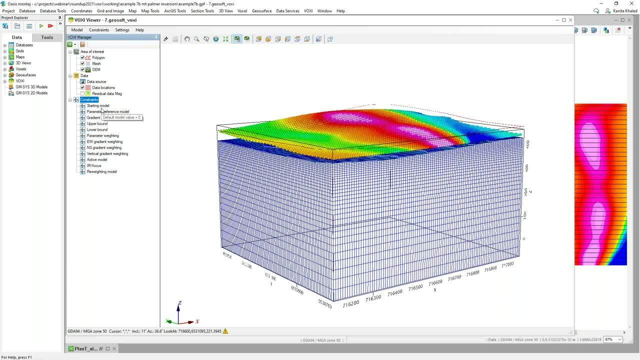
So here is our project space, or our model space,

[00:11:20.060]
if you will. And this contains in the,

[00:11:23.622]
in the small circles here,

[00:11:26.150]
those are our observed data points,

[00:11:29.100]
and those are placed within our model mesh.

[00:11:33.037]
The model mesh is our model space within which our in

[00:11:37.850]
version will, in-version results will converge.

[00:11:43.690]
And on the left-hand side here,

[00:11:45.640]
I can see a list here of constraints.

[00:11:50.320]
I have one constraint that’s in bold.

[00:11:52.620]
I’m just go ahead and turn that off for now.

[00:11:55.270]
So these are all of the possible constraints that I can add

[00:12:00.210]
to my VOXI inversion model before I press ready,

[00:12:04.170]
But right now I don’t have any active constraints.

[00:12:09.410]
If I did have an active constraint, that would be in bold.

[00:12:13.380]
So right now I have none.

[00:12:15.470]
So we could go ahead and run just this data as it is,

[00:12:20.260]
without any constraints,

[00:12:21.820]
and pressing run here would then essentially

[00:12:25.230]
upload this data onto the cloud.

[00:12:28.500]
This data would then run on the cloud and the results would

[00:12:32.000]
then be downloaded onto my computer

[00:12:34.460]
and into my VOXI project.

[00:12:36.710]
And because this is running on the cloud,

[00:12:38.780]
I could close my project up,

[00:12:40.350]
work on something else, and then return to my project once

[00:12:43.530]
it’s done.

[00:12:44.550]
And so that really allows me to free up any computing power,

[00:12:48.319]
as all the processing power is not really

[00:12:52.370]
being accessed from my local machine.

[00:12:55.470]
Okay. So for the sake of time, I have already hit run here,

[00:12:58.800]
I’ve run the model,

[00:13:00.600]
and I got my unconstrained model results.

[00:13:05.030]
So let’s take a look at the unconstrained results from,

[00:13:10.360]
from this aeromagnetic data set.

[00:13:19.350]
So here is that wireframe body again,

[00:13:22.270]
and I want to now look at my unconstrained susceptibility

[00:13:27.008]
results versus our drilling results here.

[00:13:36.890]
Okay. So here is the unconstrained susceptibility result,

[00:13:42.155]
no constraints at all,

[00:13:43.966]
and taking our, taking a first look at this,

[00:13:47.810]
it’s promising,

[00:13:50.710]
we can see that this pink anomaly, where my high is,

[00:13:54.690]
we can see that our target is recovered,

[00:13:58.330]
where it’s supposed to be, spatially.

[00:14:00.620]
So we’re off to a good start.

[00:14:03.550]
However, when I clip away at this, at this model here,

[00:14:09.900]
when I clip away at the Y axis,

[00:14:12.670]
to try to see how it corresponds,

[00:14:15.661]
we see that the geometry is not really recovered.

[00:14:21.351]
It’s a very smooth build,

[00:14:23.690]
and it’s certainly not very compact.

[00:14:25.910]
It’s not as compact as the target that I would be expecting

[00:14:29.700]
for this particular project,

[00:14:31.830]
but that’s essentially what an unconstrained result is.

[00:14:35.840]
It’s giving me the smoothest possible results,

[00:14:40.010]
so we can improve this.

[00:14:42.070]
We can definitely add a little bit more known knowledge,

[00:14:46.930]
before running our inversion,

[00:14:49.330]
and that’s where this constraint tree comes into handy.

[00:14:53.540]
This is where we’ll be adding our constraints from.

[00:14:56.820]
Okay.

[00:14:57.653]
So the first constraint we want to add is going to be the

[00:15:01.460]
upper bound constraint. And that is exactly as it sounds

[00:15:07.975]
we will right click and modify,

[00:15:09.930]
and we’ll add an upper bound constraint of one.

[00:15:14.030]
So what am I saying here?

[00:15:15.580]
By setting an upper bound constraint of one,

[00:15:18.610]
we’re saying that everywhere in this model,

[00:15:21.160]
we want to limit our inversion results to a value of one.

[00:15:25.990]
We don’t want to going higher than that,

[00:15:27.660]
because we have that knowledge of this particular area.

[00:15:31.940]
That’s what the walks in this area reflect.

[00:15:34.910]
We’ll say yes to that.

[00:15:38.186]
And similarly, you can do that for a lower bound.

[00:15:42.110]
So this is our second constraint,

[00:15:43.990]
and we’ll set this to zero, and now I have two things in

[00:15:49.240]
bold, meaning they’re both active,

[00:15:51.400]
and now we’ve applied two constraints, upper bound,

[00:15:53.990]
lower bound, with the upper bound, we set a constraint,

[00:15:57.940]
constant constraint,

[00:15:59.850]
where anywhere on our project,

[00:16:03.410]
the susceptibility value cannot be greater than one,

[00:16:07.061]
that’s the upper bound. And anywhere on our project,

[00:16:09.690]
our susceptibility cannot be less than zero.

[00:16:14.070]
So in this way, it’s very subtle,

[00:16:16.050]
but we’re guiding and pushing our solution towards values

[00:16:20.990]
That make sense from a geological perspective,

[00:16:25.510]
another really good and low effort

[00:16:30.090]
constraint is the IRI focus.

[00:16:32.830]
So this IRI focus is, again, like it sounds, it is,

[00:16:37.550]
it’s a tool that allows you to focus in your results.

[00:16:42.010]
It doesn’t require any prior knowledge of your geology or

[00:16:46.610]
the geometry of your target.

[00:16:49.330]
It stands for iterative, we’re waiting in version.

[00:16:52.200]
And what it does is it just,

[00:16:54.760]
it sharpens up an otherwise fairly smooth inversion

[00:16:59.380]
result, like the one we saw,

[00:17:01.850]
and it also improves any contact definition,

[00:17:06.085]
so this is helpful for controlling the depth of your target.

[00:17:11.850]
And it’s also very helpful in situations where you don’t

[00:17:16.253]
know any prior geological information.

[00:17:21.120]
So this is what we call a low effort, but high impact tool.

[00:17:26.590]
And by default, I have this set to two,

[00:17:29.080]
it’s a value that we know works quite well.

[00:17:37.240]
Okay. So this is now in bold,

[00:17:39.560]
so now I have three active constraints, an upper bound,

[00:17:42.990]
lower bound, and then an IRI focus.

[00:17:46.915]
The next thing is adding the geologic constraints.

[00:17:51.052]
And where is my geologic constraint coming from?

[00:17:54.920]
Well, it’s coming from this mesh that I created

[00:17:59.550]
earlier on, this wireframed body.

[00:18:02.460]
So this is what we now want to incorporate.

[00:18:06.360]
Okay. So to do that,

[00:18:09.015]
we’re going to be using the VOXI constraint builder.

[00:18:13.180]
So from constraints, I’m going to select create,

[00:18:16.710]
and then build a model.

[00:18:23.050]
And we do need an input template

[00:18:26.260]
that is going to be our mesh.

[00:18:28.450]
This is exactly this mesh here that’s been exported out.

[00:18:34.950]
And the constraint type here is going to be a parameter

[00:18:38.070]
reference model,

[00:18:43.610]
Excuse me, and for the contact here,

[00:18:47.140]
we’re going to be using the geo surface file that we created

[00:18:51.380]
from our drilling data.

[00:18:53.110]
So we know we have that mesh. And from that mesh,

[00:18:56.380]
we’re selecting the iron formation,

[00:19:00.070]
and we’re setting outside this iron formation,

[00:19:03.977]
anywhere outside this information,

[00:19:06.220]
I’m setting a value of zero, and anywhere inside this

[00:19:09.960]
formation, I’m setting a value of one.

[00:19:12.720]
So essentially, I’m taking that surface and I’m seeing,

[00:19:15.720]
and I’m guiding our inversion towards this particular value.

[00:19:21.410]
And the beauty of the constraint builder is that you could

[00:19:24.840]
keep adding more constraints, geological,

[00:19:28.030]
geologic constraints, but for our purpose,

[00:19:30.920]
we’ll just use the iron information as our main constraint.

[00:19:41.960]
That’s going to go ahead and build that parameter reference

[00:19:44.950]
model, which we can then see on our screen.

[00:19:49.470]
And if I clip away at it,

[00:19:51.280]
I can see that indeed it is that mesh. So we’re,

[00:19:54.890]
we’ve now assigned value to that particular mesh from a

[00:19:59.300]
physical property that we’ve assigned to that mesh.

[00:20:03.142]
So with the parameter reference model,

[00:20:06.304]
we don’t just supply the parameter reference.

[00:20:08.790]
It’s also paired with a weighting,

[00:20:11.230]
and this weighting allows us to define the confidence

[00:20:16.110]
in this particular reference model.

[00:20:19.250]
So that’s done through the parameter weighting here.

[00:20:24.497]
I can right click and modify,

[00:20:26.220]
and I’m setting this to a constant value of one.

[00:20:29.160]
What does that mean?

[00:20:30.820]
So this means that a value of one means that I have a very

[00:20:35.380]
high level of confidence in this parameter reference model.

[00:20:41.530]
And we have this level of confidence,

[00:20:44.750]
because we know this is real drilled data,

[00:20:49.210]
so we’re confident in it.

[00:20:52.020]
You could also use ABOXOL, which is a 3d body.

[00:20:55.740]
So that would then allow you to vary your

[00:20:59.063]
level of confidence,

[00:21:00.240]
if you had more confidence in certain areas

[00:21:03.460]
versus the other, you could specify

[00:21:05.750]
that through ABOXOL, as well.

[00:21:07.290]
But for today, we’re going to say we’re very confident

[00:21:09.570]
everywhere, and press okay.

[00:21:14.610]
And so now that is in bold,

[00:21:17.500]
so we now have the parameter reference with the mesh, and

[00:21:23.030]
we’ve given it a high weighting, or high confidence, of one.

[00:21:28.090]
Okay. Our last and final weighting today

[00:21:31.263]
will be the gradient weighting.

[00:21:36.000]
This, these three here, east, west, north, south,

[00:21:39.380]
and vertical gradient weighting.

[00:21:41.450]
So when you look at a drill core,

[00:21:44.570]
you often see really abrupt changes between two apologies or

[00:21:48.450]
your contacts, right?

[00:21:50.180]
So, you know, for example,

[00:21:52.040]
we know quite confidently that there’s likely a pretty sharp

[00:21:56.220]
contact between this iron formation and its surrounding

[00:21:59.300]
block units.

[00:22:00.980]
And if we wanted to reinforce those contacts

[00:22:05.780]
in every direction, east, west, north, south, and vertical,

[00:22:09.510]
we would have to apply the gradient weighting constraint.

[00:22:14.350]
And this constraint doesn’t require any knowledge,

[00:22:17.875]
or any information on physical properties.

[00:22:21.737]
You don’t need to know any SI values, or anything like that.

[00:22:25.140]
You don’t need any susceptibility values.

[00:22:26.850]
You’re just looking at the contacts,

[00:22:29.860]
and reinforcing the context, you’re sharpening up the edges.

[00:22:34.880]
Okay, so let’s go ahead and do that.

[00:22:36.940]
So we’re going to go into constraints, create,

[00:22:41.130]
and then gradient weight model,

[00:22:44.690]
and our input voxel is going

[00:22:46.974]
to be our parameter reference model.

[00:22:49.239]
That’s our, that’s the feature that you see

[00:22:52.190]
on the screen there.

[00:22:53.820]
And it’s asking me,

[00:22:55.520]
do you want to create this weighting in all directions?

[00:22:59.990]
You want to reinforce contacts in all directions, and I’ll

[00:23:04.340]
say yes to all directions and press okay.

[00:23:09.820]
And that would, then, go ahead and create separate waiting

[00:23:16.380]
voxels for each of those Cardinal directions.

[00:23:20.540]
So, we supplied a parameter reference model,

[00:23:23.810]
we supplied the weighting

[00:23:25.770]
for that parameter reference model.

[00:23:27.320]
We’re confident in it, and we’re saying,

[00:23:29.630]
take this reference model, and make sure you sharpen up all

[00:23:33.450]
of the contacts, and reinforce all of the edges in that

[00:23:38.110]
particular model. So, now we see these three now in bold,

[00:23:42.080]
meaning that they’re active.

[00:23:44.700]
So that was my last constraint, we have a total of

[00:23:48.682]
eight constraints,

[00:23:52.509]
eight constraints here.

[00:23:54.729]
Practically speaking,

[00:23:56.460]
I would encourage you to run the model each time you add a

[00:24:00.270]
constraint, and then inspect your result,

[00:24:03.252]
we’re going towards a solution,

[00:24:06.447]
Because if you add all of your constraints at once,

[00:24:09.930]
you’re not going to get a good understanding of how each of

[00:24:13.650]
these constraints are affecting your model.

[00:24:15.980]
So I recommend you to do this in steps, add a constraint,

[00:24:19.587]
run a model, add a constraint, run it again, evaluate.

[00:24:24.890]
And then I also recommend using the VOXI journal here to

[00:24:28.920]
track each step,

[00:24:29.810]
and keep a record of how you’re updating the model.

[00:24:35.045]
Okay. So I have all my constraints and I’m ready to run.

[00:24:40.350]
And just to be mindful of time,

[00:24:42.060]
I have run the results of this data set already.

[00:24:45.040]
So let’s go ahead and take a look.

[00:24:52.360]
So just as a reminder, this was our unconstrained model.

[00:24:58.040]
And now we can visualize the constraint,

[00:25:01.100]
constrained susceptibility result.

[00:25:06.070]
There’s our constrained model.

[00:25:09.034]
And, right away we can see that this,

[00:25:15.400]
that this model has a lot better,

[00:25:21.017]
it’s aligning with the geometry of my target a lot better.

[00:25:27.060]
And if I swing it around from this angle here,

[00:25:33.958]
I can see that it’s a lot more compact when compared to my

[00:25:36.930]
unconstrained model, right?

[00:25:40.020]
So again, there’s my unconstrained,

[00:25:42.530]
and there’s my constrained.

[00:25:45.040]
But when I start to inspect it further,

[00:25:47.980]
I do notice that there is this large volume here for the

[00:25:51.920]
susceptibility result.

[00:25:53.940]
And even after all of this constraints,

[00:25:57.472]
the susceptibility result show,

[00:26:00.330]
is showing us this large volume.

[00:26:02.380]
So, that kind of begs us to stop and question, and maybe

[00:26:06.940]
ponder whether these two bodies here

[00:26:11.421]
are potentially connected,

[00:26:14.650]
rather than the current geological interpretation,

[00:26:17.860]
which has these two bodies disconnected.

[00:26:21.710]
Even after adding our constraints,

[00:26:23.690]
we find that the theory that makes the most sense with our

[00:26:27.640]
geophysics is the one where these iron formations

[00:26:30.500]
are potentially connected.

[00:26:31.770]
And this is perhaps the time when you and your team might

[00:26:36.280]
wish to get together and discuss a new hypothesis for your,

[00:26:40.251]
for your geological model.

[00:26:43.730]
So here is our final model.

[00:26:46.572]
It led us to some new questions about our geological model,

[00:26:51.134]
and we added a total of eight different constraints.

[00:26:55.710]
So quite a rapid process with a lot of steps.

[00:26:59.950]
So I’d like to wrap up my presentation with that.

[00:27:04.340]
And I’d also like to thank you for your time.

[00:27:06.610]
If you have any questions about constraint building in VOXI,

[00:27:12.050]
I would be pleased to take them now.

[00:27:21.451]
<v ->(other speaker) Thanks Kanita.</v>

[00:27:22.390]
If anyone has any questions,

[00:27:23.430]
feel free to just type them into the chat panel.

[00:27:26.120]
I can see, we have one question already.

[00:27:31.973]
Do I need a separate extension

[00:27:34.870]
in Oasis montage for wireframing?

[00:27:39.340]
<v ->(Kanita) You do not need a separate extension in Oasis</v>

[00:27:42.530]
montage for wireframing,

[00:27:46.560]
or in target, for that matter.

[00:27:49.230]
You can wireframe right out of the 3d view.

[00:27:52.530]
Everyone who has OASIS montage has access to that, and

[00:27:56.300]
you can access it from geosurface and then wireframe.

[00:28:03.123]
<v ->(other speaker) Okay. Thank you.</v>

[00:28:05.900]
And one other question,

[00:28:10.540]
can I use drilling, or downhole data, to constrain a model?

[00:28:18.221]
<v ->(Kanita) Yes, you can use drilling data, definitely.</v>

[00:28:22.660]
So if you have either magnetic susceptibility,

[00:28:26.240]
if you’re doing a magnetic inversion,

[00:28:27.550]
or density data, if you’re doing a gravity inversion,

[00:28:32.320]
you can use those.

[00:28:33.900]
So if I go back to my VOXI model here,

[00:28:39.840]
if I go into constraints, create,

[00:28:42.650]
and then drill hole weight model,

[00:28:46.526]
this tool is what allows you to incorporate downhole

[00:28:51.540]
drilling, downhole geophysical data.

[00:28:55.160]
Something to keep in mind, when you’re putting in your

[00:28:58.340]
downhole geophysical data,

[00:29:00.460]
is that you’re measuring the absolute value

[00:29:04.690]
of the property.

[00:29:05.900]
Whereas VOXI is modeling contrasts in the property,

[00:29:11.250]
so you do need to consider whether maybe a mean background

[00:29:14.880]
would need to be removed,

[00:29:15.950]
and you can do that from this backgrounded mobile tool,

[00:29:19.420]
which we highly recommend.

[00:29:21.200]
But yeah, you can use down-hole geophysical data.

[00:29:30.791]
<v ->(other speaker) Thanks Kanita.</v>

[00:29:36.120]
At this point, I don’t see any other questions.

[00:29:42.480]
<v ->(Kanita) Okay, great.</v>

[00:29:44.390]
If you think of a question, after the demo,

[00:29:47.480]
or you have any questions in general about VOXI,

[00:29:50.750]
we’d love for you guys to get in touch,

[00:29:53.450]
you can reach me [email protected].

[00:29:58.170]
If you have any support, or workflow related questions,

[00:30:01.760]
[email protected] can also be reached.

[00:30:05.350]
And with that, I would like to end my presentation.

[00:30:07.540]
Thank you for joining and have a great weekend.