Using Economic compositing in Leapfrog Geo

Economic compositing classifies assay data into “ore” and “waste” categories, taking into account grade thresholds, mining dimensions and allowable internal dilution

Video Transcript

[00:00:07.400]
<v Narrator>Welcome to our bite-sized video</v>

[00:00:09.350]
on the economic compositing.

[00:00:11.780]
The short demonstration is designed to give you

[00:00:14.260]
an introduction to using the economic compositing tool.

[00:00:17.940]
For a detail review and guide,

[00:00:19.610]
we have a longer video available on our YouTube channel.

[00:00:23.830]
In Leapfrog, you have the option to composite drill holes.

[00:00:27.190]
Compositing is a process to reduce the variability

[00:00:29.770]
of sample sizes, that may exist in a database.

[00:00:34.230]
There are several reasons

[00:00:35.340]
why you may want to composite drill hole data,

[00:00:37.380]
and leapfrog provides different methods

[00:00:39.330]
to achieve the desired output.

[00:00:43.040]
For today’s video,

[00:00:43.873]
we are focusing on the economic composite tool.

[00:00:47.390]
The economic composite tool takes the raw assay data

[00:00:50.130]
and sets always rules based on run length grade

[00:00:53.180]
and internal dilution.

[00:00:56.160]
The output includes all waste categorical intervals,

[00:00:59.580]
as well as numeric composite intervals

[00:01:01.230]
based on a cutoff grade,

[00:01:02.690]
which can then be used to generate geological model volumes,

[00:01:05.700]
and used for statistical analysis and numeric modeling.

[00:01:10.690]
The aim is to create a reasonable mineralized envelope

[00:01:13.780]
from all intervals that have been generated

[00:01:15.550]
based on mine ability parameters,

[00:01:17.750]
in addition to a cutoff grade.

[00:01:20.930]
This is useful when geology is maybe poorly understood,

[00:01:23.880]
geology doesn’t control mineralization,

[00:01:26.470]
or when assay is the only information that is available.

[00:01:32.195]
So we’ll jump into leapfrog,

[00:01:33.550]
and we’ll start by having a look our assay data.

[00:01:39.290]
So here you can see one of our datasets,

[00:01:42.790]
where we’ve had a number of drill holes

[00:01:44.070]
intersecting mineralization.

[00:01:46.500]
In more advanced deposits,

[00:01:48.140]
you may know,

[00:01:48.973]
or want to evaluate

[00:01:49.890]
a number of mining in an economic parameters,

[00:01:51.770]
such as the impact of applying gray cutoffs

[00:01:54.330]
and minimum mining widths.

[00:01:57.440]
All compositing tools in leapfrog

[00:01:59.380]
can be found under the drill holes object,

[00:02:02.730]
in the composites folder.

[00:02:06.950]
Right click and will bring up the menu.

[00:02:08.710]
And then we can select the economic composite tool.

[00:02:12.970]
When you initially open the economic compositing tool,

[00:02:15.300]
there are a number of options available.

[00:02:17.800]
Firstly, you set the numeric value of interest.

[00:02:21.810]
In this case, we’re going to be looking today at zinc.

[00:02:25.090]
You can set rules for missing values.

[00:02:27.240]
You can either use a fixed value.

[00:02:29.670]
Sometimes things like half the detection limit,

[00:02:33.360]
or you can use an average of the enclosed intervals,

[00:02:35.500]
if your mineralization is more continuous.

[00:02:39.040]
In particularly nuggety deposits,

[00:02:41.610]
or ones with extreme outliers,

[00:02:42.970]
you can cap high grades as well.

[00:02:47.630]
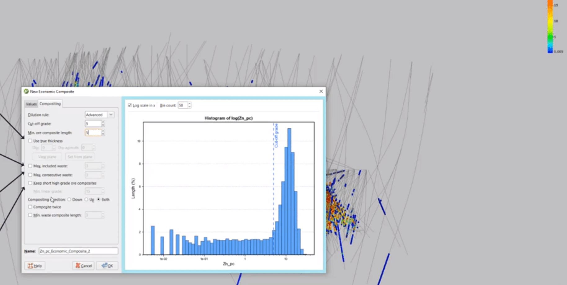
Next, we have the compositing tab.

[00:02:50.340]
There are three composting types to choose from,

[00:02:53.610]
basic, advanced and advanced plus.

[00:02:58.330]
Basic uses a simple length weighted average,

[00:03:02.320]
and will tend to produce longer waste or composites.

[00:03:06.090]
The advanced and advanced plus

[00:03:09.510]
are generally more conservative,

[00:03:11.140]
in that they provide greater control

[00:03:13.040]
over waste dilution of ore.

[00:03:14.750]
For today’s exercise we’ll pick advanced.

[00:03:18.310]
For the cut off grade, the histogram can be used as a guide.

[00:03:23.140]
There’s an option to set a standard view or lock scale,

[00:03:28.800]
and you can also adjust the number of bins.

[00:03:32.780]
Depending on what you set your cut-off grade at

[00:03:35.340]
values greater than or equal to the cutoff grade

[00:03:37.390]
is considered ore and less than is considered waste.

[00:03:42.620]
For today’s analysis we will set the cutoff at five.

[00:03:47.800]
And for the minimum ore composite length,

[00:03:50.070]
we will set the value at five meters.

[00:03:54.800]
The minimum ore interval can be designed to meet

[00:03:56.760]
a predetermined mineable ore size

[00:03:58.710]
or other factors that you may need to consider.

[00:04:02.640]
Use true thickness setting can be applied when drilling

[00:04:05.380]
is a bleak to the major trend of mineralization,

[00:04:08.130]
which can result in some…

[00:04:09.570]
sample intervals becoming much longer than the true width

[00:04:13.830]
selecting this option requires composting algorithm.

[00:04:16.790]
To composite using true thickness,

[00:04:18.610]
measured perpendicular to a specified reference plane,

[00:04:21.900]
essentially weighting the value,

[00:04:23.410]
so as not to over-represent mineralized samples.

[00:04:27.640]
Max included waste is an optional threshold.

[00:04:30.230]
The constraints is the total length of waste

[00:04:31.960]
that can be accumulated within an ore composite.

[00:04:34.900]
Increasing this value will permit

[00:04:36.950]
greater dilution of ore with waste

[00:04:39.310]
before the candidate ore section will be rejected.

[00:04:43.220]
Max consecutive waste is an optional threshold for basic,

[00:04:46.950]
and advanced dilution rules,

[00:04:48.680]
but it is required for the advanced plus.

[00:04:51.630]
It constraints the length of the consecutive end force

[00:04:53.980]
classified as waste that can be considered

[00:04:56.340]
for addition to an old composite.

[00:05:00.620]
keep short high grade or composites is an option that allows

[00:05:04.070]
all composites less than the minimum length to be included.

[00:05:08.540]
This is provided at the minimum linear grade is exceeded.

[00:05:12.100]
Compositing direction,

[00:05:13.480]
just determines which way the algorithm runs

[00:05:16.780]
up or down the hole.

[00:05:19.180]
And when you use an advanced,

[00:05:20.080]
advanced plus, both is selected as default.

[00:05:24.420]
compositing twice,

[00:05:26.000]
will run the compositing process a second time

[00:05:28.130]
after the first pass,

[00:05:29.510]
which can sometimes help to smooth out and the results.

[00:05:34.540]
Once we’ve set a cut-off grade of 5%

[00:05:37.640]
and a minimum length of five,

[00:05:39.950]
I’m going to leave the other ones as default,

[00:05:43.150]
and we’ll just pick an appropriate name

[00:05:45.960]
for our composite table.

[00:05:54.680]
click okay and let this run.

[00:05:59.670]
Once this is processed,

[00:06:01.600]
we now have the new table in our composite folder.

[00:06:06.730]
If we double click to look at the table,

[00:06:08.130]
we can see it brings up an overview of the data available.

[00:06:14.040]
To quickly run through these,

[00:06:15.350]
status is the category, is defined as ore or waste

[00:06:18.950]
based on our parameters.

[00:06:21.270]
Using the same column gives you the weighted average grade

[00:06:24.550]
of that interval.

[00:06:26.440]
The true length is the linear length of that interval.

[00:06:30.980]
Linear grade is the average grade times by the true length.

[00:06:37.210]
The dilution true length,

[00:06:39.780]
is the total length of any diluting intervals.

[00:06:42.600]
i.e, intervals that fall below the cutoff we’ve specified.

[00:06:46.560]
Your dilution linear grade, is the weighted linear grade

[00:06:50.410]
below the cutoff material times by the length

[00:06:53.748]
and the percentage missing,

[00:06:56.220]
is the percentage of missing samples within the composite.

[00:07:02.610]
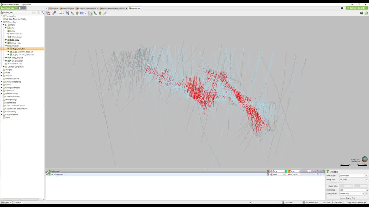
If we load, our composite table onto the scene,

[00:07:08.780]
we can turn off the assays, and have a look at the results.

[00:07:14.950]
So you can see we had the legend.

[00:07:19.350]
That the composting tool has gone through

[00:07:20.780]
and classified our drill holes

[00:07:22.410]
into waste in blue, and ore intervals in red.

[00:07:30.390]
If we turn off the waste,

[00:07:35.270]
we can start to get an idea of the trend,

[00:07:38.830]
and the direction of the mineralization.

[00:07:49.290]
To have a look at this in a bit more detail

[00:07:50.690]
what we’ll do is,

[00:07:51.523]
we’ll focus in on one particular drill hole.

[00:07:55.190]
If I click on my ore interval,

[00:07:58.260]
I get the same statistics that we looked at on the table.

[00:08:01.550]
So in this case,

[00:08:02.383]
I can see that my ore interval is 55.1 meters long

[00:08:06.120]
and average grade of 12.72%.

[00:08:10.340]
Within this ore interval, I have 2.5 meters of dilution,

[00:08:17.180]
and we can see that 2.5 meters is probably this

[00:08:21.550]
sample sits in here.

[00:08:24.310]
I can color this by the same discreet color map

[00:08:28.010]
to see what falls above and below.

[00:08:31.060]
We can then start to understand the impacts

[00:08:33.370]
of these decisions through numerical models

[00:08:35.470]
or use the category data to model domains.

[00:08:38.760]
For a reasonably complex topic.

[00:08:40.330]
This is a very brief overview.

[00:08:42.350]
As mentioned at the start of the video,

[00:08:43.840]
we have a more detailed discussion around the settings

[00:08:45.980]
and processes on our YouTube channel,

[00:08:47.810]
which I’d recommend you watch.

[00:08:49.010]
If this is something that may be of value to you.

[00:08:51.990]
Thanks very much for joining.