Unlocking Value For Geotechnical Engineers in Leapfrog Geo

The webinar will cover an introduction to Leapfrog Geo as well as an overview of the key functionality that can aid geotechs in their daily workflows.
This includes:

• Importing and viewing drillhole data
• Building a simple geotechnical domain model
• Creating fault surfaces and generating fault domains
• Importing and viewing structural data
• Creating numeric models of RQD or RMR data

Overview

Video Transcript

[00:00:00.400]<v ->Hello everyone.</v>

[00:00:01.250]Welcome to today’s webinar.

[00:00:03.650]Thanks for joining me today.

[00:00:04.730]My name is Sophie Tie and I’ll be running today’s webinar,

[00:00:08.610]unlocking value for Geotechs and LEAPFROG-GEO.

[00:00:12.010]I recently joined Sequence Asia Pacific team in Perth

[00:00:14.900]as an engineering geologist.

[00:00:16.700]My background is both in the civil industry

[00:00:18.367]and the mining industry

[00:00:19.730]predominantly in gold and base metals.

[00:00:23.240]So to begin today, I will introduce Sequent as a company

[00:00:27.080]and then go into a bit more about

[00:00:28.810]how Leapfrog can and is being used in the

[00:00:30.980]Geo-technical engineering space.

[00:00:33.500]Then we’ll move into a demonstration of the software

[00:00:35.660]to show some useful features and workflows.

[00:00:38.490]So you can see how our products can and are being used

[00:00:40.770]to support Geotechs in the mining industry.

[00:00:43.800]This presentation will be quite high-level

[00:00:45.680]and isn’t an in-depth demonstration

[00:00:48.510]of a specific how-tos within the software.

[00:00:51.980]For training in the software,

[00:00:53.710]or for assistance with your products,

[00:00:55.800]please contact your local Leapfrog office.

[00:00:59.080]So Leapfrog, the software application,

[00:01:00.900]most people are familiar with already

[00:01:03.040]is a package with the visualization

[00:01:04.930]and the modeling is completed.

[00:01:07.360]This includes both Leapfrog-geo

[00:01:09.470]our implicit modeling software for geological modeling

[00:01:12.760]and Edge and additional model,

[00:01:14.580]which unlocks the estimation functionality.

[00:01:17.430]However, Leapfrog is just one component

[00:01:20.060]within the greater sequence solution.

[00:01:23.270]This slide illustrates how the sequence suite of products

[00:01:26.160]establish and sustain a continuous flow of communication

[00:01:29.900]that benefits the entirety of your organizations

[00:01:32.420]and even groups beyond that who ultimately impacts

[00:01:35.010]the decision making process.

[00:01:37.830]So at the top of this figure we have View.

[00:01:41.870]View is a free collaboration tool

[00:01:43.950]ingrained within Leapfrog that allows users

[00:01:47.060]to visualize, discuss, and share 3D models.

[00:01:50.950]For example, on the decision-making level,

[00:01:53.590]there are a multitude of impacting factors

[00:01:55.870]that leads to a final decision.

[00:01:58.000]To be heard and considered the information needs to be

[00:02:00.390]communicated quickly, clearly,

[00:02:02.690]and as intuitively as possible.

[00:02:04.830]And often to people outside the organization as well.

[00:02:08.160]This is where View shines.

[00:02:11.510]Moving down to the center of this figure we have Central.

[00:02:15.640]Internally when stepping into the more technical realm,

[00:02:18.590]the data volume that needs to be shared and understood

[00:02:21.050]is much larger.

[00:02:22.320]Therefore, a different system, IA central

[00:02:25.360]can be accessed for collaboration and allows

[00:02:27.740]not only for the visualization of modeling data,

[00:02:31.050]but also its safekeeping and organization

[00:02:34.190]facilitating the audibility of the company.

[00:02:38.150]Towards the end of today’s webinar,

[00:02:39.830]we will take a brief look at the value that central provides

[00:02:43.140]and how more and more Geotechs are using it,

[00:02:45.550]particularly for its auditability function,

[00:02:48.360]as well as for accessing geological models

[00:02:50.750]as a starting point for geotechnical models.

[00:02:55.570]Then on the high technical end at the bottom of this figure

[00:02:58.250]sits the modeling software,

[00:03:00.150]which is directly connected to central

[00:03:02.060]in all geo-science information used in the modeling process.

[00:03:05.580]By having instant access to the latest information,

[00:03:08.000]both about data, as well as intelligence exchange,

[00:03:11.350]the communication cycle is complete.

[00:03:16.410]The geo-technical model is widely considered to be

[00:03:20.030]the cornerstone of any underground

[00:03:22.050]or open-pit mining geotechnical design.

[00:03:24.880]It provides the basis for developing geotechnical domains

[00:03:28.930]and analysis inputs,

[00:03:30.810]meaning it is directly linked to the confidence

[00:03:33.510]and reliability of your design.

[00:03:36.870]A geotechnical model combines and considers all

[00:03:40.220]geotechnical data, which includes

[00:03:42.770]geological, structural, hydro geological

[00:03:46.260]and geo-mechanical data to create

[00:03:48.840]a powerful tool that can be used to inform

[00:03:51.264]a myriad of geotechnical considerations

[00:03:54.970]regarding all stages of both open pit

[00:03:57.360]and underground mining operations.

[00:04:01.260]Essentially, the geo-technical model forms the basis

[00:04:03.660]of decisions surrounding and these are not limited to;

[00:04:06.850]pit geometry, slope, and better angles

[00:04:09.530]mining method, and equipment selection.

[00:04:12.540]It also plays a factor in virtually all other

[00:04:15.490]strategic planning decisions.

[00:04:18.210]So with this in mind, here are some of the major benefits

[00:04:21.450]our geotechnical users are experiencing

[00:04:23.930]when using Leapfrog-geo for getting this job done.

[00:04:28.410]One of the major benefits is the ability to have

[00:04:31.100]all your geotechnical data in one place.

[00:04:33.650]This includes your geotech logs drillholes,

[00:04:36.000]RQD data, pit wall, or window mapping,

[00:04:38.940]lab testing, photogrammetry etc.

[00:04:44.706]Then not only is it easy to import this data,

[00:04:47.210]having it all in Leapfrog makes

[00:04:49.300]visualization and analysis straightforward.

[00:04:53.770]Being able to integrate multidisciplinary data sets

[00:04:58.050]is also a huge advantage as it removes the need to have

[00:05:01.140]related relevant data spread across multiple packages.

[00:05:05.200]And this ensures all is considered,

[00:05:07.210]and that it is considered holistically

[00:05:09.140]when undertaking modeling and analysis.

[00:05:12.340]No data gets left out.

[00:05:14.760]Finally, the rapid 3D modeling functionality

[00:05:17.750]is a game changer.

[00:05:20.020]Leapfrog uses the our B if interpolant

[00:05:22.930]to quickly generate surfaces which means

[00:05:25.460]you can run and re-run multiple iterations,

[00:05:28.360]and we add new data.

[00:05:30.000]The model is updated quickly.

[00:05:32.776]Data Sources.

[00:05:34.600]So geotechnical data can be collected from

[00:05:37.280]a plethora of sources and many different formats,

[00:05:40.810]in terms of leapfrog.

[00:05:42.240]The most relevant data source is going to be

[00:05:45.010]structural data and rock mass classification data.

[00:05:49.080]Some of the more common sources of this data are

[00:05:52.100]photogrammetry, core logging, underground mapping,

[00:05:54.700]pit wall mapping, bench case inspections, field scanning.

[00:05:58.600]And this data can all be applied directly

[00:06:00.960]to your leapfrog models to implicitly generate surfaces.

[00:06:04.840]And then dynamically update these as new data is added.

[00:06:09.530]In the geotech space,

[00:06:11.130]there is also other data and work going on across a range

[00:06:14.890]of other areas or other software packages.

[00:06:18.730]These can include things like lab testing results,

[00:06:21.410]seismic data, swiped stability models, stress models.

[00:06:25.440]So any parameter that has an X, Y or Z value or sorry,

[00:06:30.110]an X, Y, and Z value can be brought into Leapfrog

[00:06:35.030]and viewed as point data or coated points.

[00:06:39.250]And this gives you a platform to view

[00:06:42.140]all the relevant data in one place

[00:06:44.600]alongside all the other relevant data.

[00:06:50.310]Okay, Leapfrog for geotechs.

[00:06:52.530]So today we’ll be covering some of the basic functionality

[00:06:56.800]in Leapfrog used to create a geotechnical model.

[00:07:00.790]And we’ll go through a workflow for creating

[00:07:03.410]a geotech model in Leapfrog.

[00:07:06.300]The fundamental idea of making a geotech model

[00:07:09.020]is similar to that of creating a geological model,

[00:07:11.440]and that is getting your domaining correct.

[00:07:15.670]So today’s workflow will look something like this.

[00:07:18.580]Firstly, we’ll use existing structural and geological models

[00:07:23.230]as the starting point for domaining.

[00:07:26.180]Then we will look at using some of the

[00:07:28.870]cool statistical tools in Leapfrog,

[00:07:31.830]to see if these domains require further sub-domaining.

[00:07:35.380]We will then look at creating a numeric model

[00:07:37.730]within these domains to create to estimate RQD.

[00:07:42.600]And then finally, we will look at some outputs

[00:07:45.810]that could be used for geotechnical design.

[00:07:49.940]Finally, this slide outlines

[00:07:51.700]what we’ll be covering in our demonstration.

[00:07:54.970]So we’ll begin by importing

[00:07:56.620]and using some tools to view drillhole data.

[00:08:00.100]Then we will look at a couple of ways

[00:08:02.330]to drill and make fault surfaces, and some fault domains.

[00:08:06.240]And then we’ll go on to view

[00:08:08.390]and analyze our structural data.

[00:08:11.630]And here’s a couple of cool tools to demonstrate

[00:08:13.995]highing further sub-domain your geotechnical domains.

[00:08:19.430]We’ll look at generating a simple geotechnical domain model.

[00:08:24.520]And finally, we’ll look at creating a numeric model

[00:08:28.980]based on RQD data.

[00:08:31.840]So, let’s jump into it.

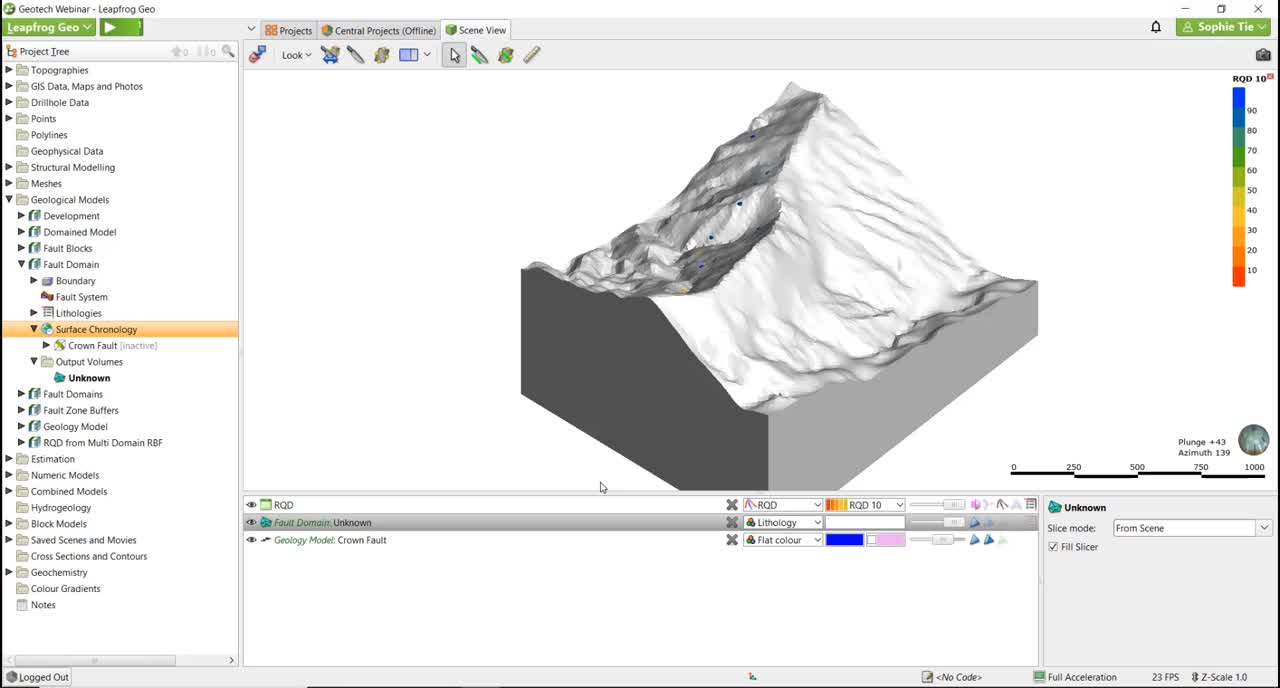
[00:08:34.120]To start with, I’m just going to quickly run through

[00:08:36.220]the Leapfrog-geo main window,

[00:08:39.360]just for those of you who might not have seen it before.

[00:08:41.840]So at the top left corner we have the menu,

[00:08:44.550]and this is where we can open projects, create new projects,

[00:08:47.740]save a copy and have it play around with how settings.

[00:08:51.640]Along the top we have the toolbar

[00:08:54.690]and you’ll see me using

[00:08:55.870]some of these buttons throughout today’s webinar.

[00:09:00.690]In the left-hand panel here

[00:09:02.350]we have the project tree, which has a

[00:09:04.540]top level list of standard folders and objects.

[00:09:07.910]The project tree is where you import your data

[00:09:10.750]and where you work with your data.

[00:09:13.350]The processing panel is at the top here on the right

[00:09:15.790]of the Leapfrog-geo main menu button.

[00:09:18.160]And it’s opened by clicking on the button

[00:09:20.030]to the right of it.

[00:09:21.740]The button is inactive when there are no tasks running

[00:09:24.380]and it’s green when tasks are running.

[00:09:27.880]In the center our screen, we have the same view,

[00:09:30.060]which is where objects appear,

[00:09:32.540]when we edit from the project tree.

[00:09:35.200]To add an object to the project tree,

[00:09:38.330]we just select then drag and drop.

[00:09:42.920]The shapes list below the same view lists

[00:09:45.670]all of the objects that are active

[00:09:46.980]or visible in the same window.

[00:09:49.560]And finally, down at the bottom left corner,

[00:09:51.620]we have the status bar.

[00:09:53.880]The coordinates that appear in the status bar via

[00:09:57.850]show the location of the mouse cursor

[00:09:59.870]when it is over an object in the same window.

[00:10:05.330]So for today’s webinar, we’re just going to say that

[00:10:06.970]we’ve been given this geology model by the geology team.

[00:10:12.530]Right, so we’ll just move on to

[00:10:15.860]importing and varying our drillhole data I think.

[00:10:20.760]So I’m just going to bring in the drillholes

[00:10:22.430]that have been logged for lithology.

[00:10:28.820]Cool.

[00:10:29.653]So he’s a legend up here and we can see what lithologies

[00:10:35.700]have been used to generate the geological model.

[00:10:39.130]So we can see that we have recent and blues

[00:10:41.510]sitting in the top of the drillholes.

[00:10:44.520]Dacite in purple early diorite,

[00:10:48.600]and yellow, and basement, and green.

[00:10:53.090]There’s also a fault code here in Edge,

[00:10:55.510]which is where the geologists have logged fault zones.

[00:11:00.370]And there’s a few ways you can sort of display

[00:11:04.120]and visualize your data and the same.

[00:11:07.620]So I’m just going to display the geological model again

[00:11:10.130]that’s been generated from we using this drillhole data.

[00:11:15.608](keyboard typing)

[00:11:20.040]Cool, so we can see that there is a thin layer of cover

[00:11:23.830]at the top, which is been logged as recent.

[00:11:27.860]And then underneath that we have our basement and dacite,

[00:11:34.960]and that’s been intruded by our early diorite.

[00:11:41.100]We also have two faults

[00:11:44.560]that have been defined using the fault logging.

[00:11:48.900](keyboard typing)

[00:11:57.880]Which we can see just in there.

[00:12:01.560]Cool, so that’s kind of how we view it

[00:12:03.150]and look at our data, our drillhole data.

[00:12:06.310]Now we’re going to look at faults.

[00:12:08.580]So there’s two common methods for delineating fault zones,

[00:12:14.810]and we will be using our RQD data to do this today.

[00:12:21.921]So if we just bring in our,

[00:12:23.630]oh wrong one, sorry.

[00:12:26.190]Let’s bring in our RQD data, cool.

[00:12:30.500]So here you can see the RQD logging

[00:12:33.920]with the reds and oranges indicating areas of low RQD

[00:12:37.910]and the blues and greens indicating areas of high RQD.

[00:12:44.390]So once again, another way of viewing it.

[00:12:45.920]And there’s also the option to add a value filter

[00:12:50.900]down in the bottom right corner in the properties panel.

[00:12:55.280]So you might want to do this if you want

[00:12:56.380]to highlight say your law of values.

[00:13:00.140]You can also create your own color maps down here

[00:13:04.280]in the shapes list.

[00:13:07.990]Cool. So I’m just going to bring in the ground fault.

[00:13:14.040]Cool. So here we can see this fault plane

[00:13:17.420]that the geo’s have mapped,

[00:13:20.210]and we can say when we overlay it onto the drilling,

[00:13:22.200]it kind of well, it coincides with the lower RQD areas.

[00:13:28.660]So you can see the faults aligning with that RQD data.

[00:13:35.830]Cool. So the first way we’re going to model a fault

[00:13:38.910]or a damaged domain, is by using distance buffers.

[00:13:43.540]So we’re going to create distance buffers

[00:13:45.810]around this fault plane here.

[00:13:48.168]And this is really beneficial when you want to get an idea

[00:13:50.460]of what the distribution of the RQD is

[00:13:53.510]at different intervals away from the fault.

[00:13:57.728](keyboard typing)

[00:14:06.431]Cool. Okay.

[00:14:08.050]Oh, a bit of a delay.

[00:14:09.940]Cool.

[00:14:10.830]Okay. So now we’re looking at our RQD drilling still

[00:14:14.600]and a distance buffer that’s created.

[00:14:16.880]That’s been created around that blue fault plane.

[00:14:20.807]And if I just take a slice perpendicular through here.

[00:14:27.500]Oh, that’s a bit of a delay.

[00:14:30.420]We can see our fault plane here at the center,

[00:14:32.560]this blue one.

[00:14:34.290]And then into the distance buffers

[00:14:35.740]that have been created at 10 minute intervals,

[00:14:38.930]moving away from that fault plane.

[00:14:42.340]So once we’ve created these distance buffers,

[00:14:44.420]it’s possible to back flag

[00:14:45.980]the distance buffer model onto the drilling

[00:14:48.740]and use that to have a look at some statistics.

[00:14:51.670]This is extremely useful as it allows you to see

[00:14:54.659]what the RQD is doing in each buffer zone.

[00:14:58.170]So I’m just going to right click on my merged table,

[00:15:04.300]and I select statistics,

[00:15:05.510]and I’m going to go with a tableau statistics.

[00:15:09.220]Cool. So here we can see some basic stats

[00:15:12.420]for our RQD values within those distance buffers

[00:15:16.130]we made around our fault plane.

[00:15:18.960]So count as a total number of individual samples

[00:15:23.090]in each envelope, which distance buffer.

[00:15:25.840]Length is the total number of samples.

[00:15:28.510]So the total. Okay length is the total length of samples

[00:15:33.590]and main is the main RQD.

[00:15:37.470]So we can see that the RQD

[00:15:40.900]or the main RQD

[00:15:42.010]within 10 minutes of the fault is around 45, 46

[00:15:46.600]at 20 meters, it’s about the same and so on.

[00:15:50.680]And then we come to 50 meters

[00:15:54.810]away from our fault and RQD jumps from about 55, up to 70.

[00:16:00.110]So from this, we can infer that the fault zone

[00:16:02.320]has a zone of influence of about 45 or 50 meters

[00:16:06.260]from the crown fault, fault plane.

[00:16:11.760]Cool.

[00:16:13.850]So what we’ll do now is take a look

[00:16:16.280]at the second method of defining a fault zone.

[00:16:20.330]So we’ve looked at distance buffers,

[00:16:21.850]and this time we’re going to use the interval select total.

[00:16:26.260]So if I just remove these buffers,

[00:16:31.200]you can see that we’ve now got the RQD drilling

[00:16:35.280]and the fault plane.

[00:16:36.780]And if I just pan through this and section view,

[00:16:41.539]and we can see that there are areas of the fault plane

[00:16:44.610]that don’t necessarily honor or reflect

[00:16:51.940]the RQD data that we’re looking at.

[00:16:58.280]So I guess the fault plane is like a lot smaller

[00:17:01.510]and one thing we would expect, I fault zone

[00:17:03.960]or a fault domain to be based on this area

[00:17:07.310]of low RQD values.

[00:17:09.560]So for the next option, we’ll,

[00:17:12.000]we’re going to use the interval select total

[00:17:13.520]to a model a fault domain.

[00:17:16.110]By selecting the areas of low RQD

[00:17:18.240]that we believe are associated with the fault.

[00:17:21.970]So using the interval select tool,

[00:17:25.379]is really, really beneficial when you want to accurately

[00:17:28.010]delineate zones that vary in width.

[00:17:31.030]And we know if this is generally the case of faults

[00:17:33.220]that almost never uniform plane and structures

[00:17:35.790]and estimos that can be discontinuous

[00:17:37.640]and might have localized zones of wider or thicker

[00:17:40.570]or thinner shearing or appreciation.

[00:17:44.880]So, yeah,

[00:17:45.713]so what we’ll do is we will go into RQD here and

[00:17:52.210]select a new interval selection,

[00:17:56.390]just call that fault.

[00:17:59.790]And then what we’ll do is,

[00:18:02.890]oh it’s still thinking.

[00:18:07.340]We’ll just go through here and

[00:18:10.780]select the areas of low RQD.

[00:18:16.066](keyboard typing)

[00:18:21.514]That we believe are associated with our fault.

[00:18:27.930]So we’ll just keep penning through until we’ve got them all.

[00:18:33.520]And it could be as well, maybe

[00:18:36.520]down here.

[00:18:39.401](keyboard typing)

[00:18:53.924]And yeah so.

[00:18:55.540]What would do is we’d,

[00:18:57.171]we’d step through the whole model like this

[00:18:59.860]selecting the areas that we’d like to

[00:19:04.510]represent our faults on.

[00:19:07.350]And then what we’ll do is we’ll just assign these to

[00:19:11.480](keyboard typing)

[00:19:13.445]a new fault.

[00:19:16.920]Okay.

[00:19:17.753]And then we would save it.

[00:19:20.220]So you would, you’d go through

[00:19:22.320]and do this through your model.

[00:19:23.727]Selecting all of the intervals that you want to be included

[00:19:26.450]in your fault domain.

[00:19:29.120]Cool, so now I’m just going to create,

[00:19:33.240]a new model,

[00:19:35.010]that’s going to be comprised of these fault domains.

[00:19:38.750]So to create a new model, just go new geological model,

[00:19:47.339]maybe fault selection,

[00:19:48.960]change my surface resolution.

[00:19:53.129]And close our RQD.

[00:19:56.031](keyboard typing)

[00:20:20.180]Cool.

[00:20:21.500]So I’ve just brought in this output volume here.

[00:20:27.618]So we can see how the model has been set up.

[00:20:29.480]This is the output volume,

[00:20:30.770]and this indicates what the extent of the model will be.

[00:20:33.550]And then when we go on to build our model,

[00:20:35.240]we’ll create services that will then activate as volumes.

[00:20:38.100]And these volumes will be generated by being

[00:20:40.080]essentially cut out of this shape.

[00:20:43.140]So this will result in a collection of close message

[00:20:46.360]meshes or air type volumes.

[00:20:50.340]So we’re going to use the vein modeling tool

[00:20:52.400]for the fault we’ve just selected those intervals for,

[00:20:56.470]and I’ve actually gone through and selected those intervals

[00:20:59.080]prior to this webinar,

[00:21:00.070]just because it would have taken too long to do live.

[00:21:01.710]So just, but just so you get the idea.

[00:21:04.610]So we’re going to surface chronology

[00:21:06.620]a new vein from base lithology.

[00:21:10.220]Yep. Crown fault, crown fault.

[00:21:12.710]Okay, cool.

[00:21:14.950]So the vein modeling tool is useful when you want to

[00:21:18.310]model two sets of contact points above and below

[00:21:21.240]the unit that you’re modeling.

[00:21:23.120]So it will create a hanging wall set

[00:21:24.650]and a foot wall set of contact points.

[00:21:28.610]Cool. So that’s done so we can see how quickly,

[00:21:34.480]how quick it is to create a new volume

[00:21:36.470]that represents this fault domain,

[00:21:39.260]which encompasses the intervals that we selected,

[00:21:41.630]or that I selected earlier.

[00:21:46.090]Cool.

[00:21:47.210]So now we have a more accurate volume representing

[00:21:51.290]our fault domain.

[00:21:53.870]So it’s possible to back flag this version

[00:21:56.350]of the model onto the RQD drilling.

[00:21:58.640]And this is useful because it enables you to review

[00:22:01.150]your RQD data against this newly generated volume.

[00:22:06.100]So to do this I’ll just open another table of statistics,

[00:22:11.457](keyboard typing)

[00:22:15.181]statistics I’m going to go for a table of statistics again.

[00:22:19.490]Cool. So here we can see our lithologies and the crown fault

[00:22:22.870]we just modeled against the main RQD values.

[00:22:28.151]So we can see the main RQD for crown faults about 46,

[00:22:31.670]which is a lot, lot lower than the,

[00:22:35.390]the other surrounding lithologies.

[00:22:39.610]Cool.

[00:22:42.510]So moving on to importing and viewing structural data.

[00:22:48.580]So in addition to the geology and RQD,

[00:22:52.690]we’ve looked at so far.

[00:22:53.523]This data set also has five holes

[00:22:57.160]that have been logged for Q parameters.

[00:23:01.700]So I’ll just put those in there.

[00:23:03.350]So structural measurements are shown as discs in Leapfrog.

[00:23:06.450]Each of these structured disks,

[00:23:09.150]we have a dip dip as a myth, joint alteration,

[00:23:13.020]and joint roughness measurement.

[00:23:15.380]These measurements, obviously from our drillholes,

[00:23:18.400]but it’s just as easy to bring in field mapping data

[00:23:20.620]or structural measurements

[00:23:22.310]that have been taken from pitwall mapping or window mapping.

[00:23:27.200]So we’re going to have a look at this data

[00:23:28.810]on a stereonet to start with

[00:23:32.000]Leapfrog has a built in stereonet,

[00:23:35.130]which is a really handy visual tool.

[00:23:36.960]And of course, there’s a benefit of it being

[00:23:38.900]in the same piece of software as your model

[00:23:40.537]and all your other data.

[00:23:41.950]So no need to nip back and forth,

[00:23:43.350]or do a data entry and another piece of software.

[00:23:47.490]So,

[00:23:48.323]stereonets are in the structural modeling folder

[00:23:51.890]in the project tree

[00:23:55.390]and what we’re looking at,

[00:23:58.960]here are the structural measurements

[00:24:00.580]from those five geotech holes

[00:24:03.410]that we could easily bring in out field mapping data

[00:24:05.360]in the same way.

[00:24:07.040]Cool. So in the stereonet window,

[00:24:08.440]we have the option to add additional data up here.

[00:24:13.940]We can offer either Bingham or Fisher statistics.

[00:24:17.660]We can export the stereonet as a PDF

[00:24:22.180]and under options we can select between

[00:24:25.700]an equatorial polar stereonet type equal area

[00:24:30.380]or equal angle projection.

[00:24:32.720]And then, you know,

[00:24:34.610]we can play around with the spacing

[00:24:35.600]of the XCs and the labels.

[00:24:39.537]Okay. So over here we have the properties panel,

[00:24:42.690]so we can choose to display our structure measurements

[00:24:45.570]as poles to planes, or we can have the planes if we want,

[00:24:50.670]maybe here, oh the delay.

[00:24:53.849]And we could even have our default contours.

[00:24:59.810]Cool.

[00:25:00.643]So we’re going to go through the process

[00:25:03.010]of defining our own joint sets today.

[00:25:10.543]I’m just going to call this (keyboard typing) joint set.

[00:25:14.516]Okay.

[00:25:15.810]So you will note how this,

[00:25:17.290]the colour of the stereonet changes.

[00:25:22.787]Here we go.

[00:25:23.620]And I’m just going to click around here

[00:25:26.280]and select all of the measurements that I believe

[00:25:31.788]to be the same joint set and

[00:25:34.970]assign them to a new joint set.

[00:25:39.292]I’ll call that joint set one.

[00:25:41.050]Cool, cool.

[00:25:43.790]So if I just undock this stereonet window

[00:25:47.210]and show you what we’ve got going on

[00:25:49.970]in the same view at the same time.

[00:25:53.250]We can see that the joints I’ve attributed as JS one,

[00:25:58.460]which now is red in the stereonet,

[00:25:59.920]and also red in the same view.

[00:26:01.510]So it’s totally interactive.

[00:26:05.520]So if I just continue now

[00:26:08.760]for the second

[00:26:12.210]joint set, you can see how these ones are getting selected

[00:26:15.630]in the same view.

[00:26:20.250]I’ll call that JS two.

[00:26:22.470]Cool.

[00:26:23.303]So you would repeat this until you have all

[00:26:26.070]of your joints is defined.

[00:26:28.010]So 1, 2, 3, 4, 5, plus the other one’s assigned to random,

[00:26:34.490]I’m going to just flick over to one I did before.

[00:26:39.046]I will just discard that.

[00:26:40.420]And here is the one that I prepared earlier.

[00:26:42.510]So you can see I’ve got five joint sets

[00:26:44.730]and I’ve just assigned the remaining ones

[00:26:46.840]to category code category called random for now.

[00:26:51.035]So there’s a few additional visual tools

[00:26:53.950]such as showing

[00:26:56.320]the average plane of each group of measurements.

[00:27:02.330]And it’s also possible to view this here unit in 3D.

[00:27:07.260]So we can have the head view here or go back to

[00:27:10.750]our same view where’s our structural

[00:27:16.160]measurements here they are.

[00:27:19.120]And I’m just going to bring my stereo net into the same view.

[00:27:23.590]Cool.

[00:27:26.210]Yeah. So this is just a really awesome tool

[00:27:27.920]for visualizing your data on the stereonet

[00:27:30.790]and insert your orange space at the same time.

[00:27:36.700]So earlier I said that lithology is often a starting point

[00:27:41.000]for geotech domains or the lithological or geological model

[00:27:44.410]is a starting point for the geo-technical domain model.

[00:27:50.016]So yeah,

[00:27:50.849]because it’s reasonable to assume that different rock types

[00:27:53.090]or different lithologies have different properties.

[00:27:55.690]So what we’re going to do now is evaluate the geological

[00:27:58.830]model onto the structural measurements in those drillholes.

[00:28:02.690]And this is useful as it allows you to see

[00:28:05.200]what lithology the structural measurement was taken in.

[00:28:10.150]So we’ll just go back to our 2D stereonet

[00:28:13.350]and have a look at what joint sets have occurred

[00:28:20.250]and which lithology.

[00:28:25.610]Cool. So in joins set one,

[00:28:26.960]which was down here appears to have occurred

[00:28:29.350]in the early diorite at the dacite and the basement.

[00:28:32.890]Joint set two here is predominantly in the dacite.

[00:28:36.310]Joint set three is pretty much joining in the early diorite.

[00:28:40.839]Joint set four is only the basement, and joint set 5.

[00:28:46.630]Yeah. Predominantly in the diorite again.

[00:28:48.260]If you’re dacite measurements, it looks like as well.

[00:28:52.470]Cool.

[00:28:53.303]So we can go one step further by a query

[00:28:55.600]by applying query filters.

[00:28:57.550]So for example,

[00:28:58.570]if I turn on this query filter for a basement,

[00:29:06.883]we can see that there are two joint sets in the basement,

[00:29:08.944]joint set one and joint set four,

[00:29:11.500]and then there’s remaining random sort of scattered around.

[00:29:14.450]And then for the dacite,

[00:29:19.780]we can see we’ve got three joints sets.

[00:29:22.940]One, two, and I think it’s five that one there.

[00:29:29.000]Cool. So now that we’ve started quantifying this,

[00:29:31.640]we can move on to start to quantify a J in value

[00:29:35.830]based on the available data.

[00:29:40.400]Let’s closed and do the same.

[00:29:43.350]So we’re going to move on to sub domaining now,

[00:29:46.010]and this section is really helpful for when you are

[00:29:49.320]evaluating if you should further divide up existing domains

[00:29:54.760]into sub domains to reflect your data.

[00:29:57.840]So so far, we’ve domained at the fault zone

[00:30:01.030]and we’ve got the lithology domains from the,

[00:30:03.340]from the geological Model.

[00:30:05.020]And now we’re going to see if there are multiple domains

[00:30:08.130]within these lithologies or a further domaining

[00:30:11.740]within the lithologies is required.

[00:30:14.320]And to do this, we’ll be using a combination

[00:30:16.590]of what we found earlier in our stereonets

[00:30:18.760]and some statistical views, sorry.

[00:30:22.530]Some statistical tools, I think I said views,

[00:30:27.040]I think I said views.

[00:30:27.873]I should’ve said statistical tools.

[00:30:29.880]Cool.

[00:30:32.947]So let’s bring in this one here.

[00:30:38.091]And geological model transparent.

[00:30:43.240]Okay, cool.

[00:30:44.073]So we can,

[00:30:44.906]what we’re going to do is look at how the three lithologies

[00:30:52.320]basement dacite and early diorite,

[00:30:55.640]vary across the 3 1, 2, 3, fault blocks.

[00:31:01.480]This could also be applied to weathering profiles

[00:31:03.770]or any type of spatial variability

[00:31:06.730]that might exist within the model.

[00:31:08.370]So if we look at the combined model,

[00:31:12.051](keyboard typing)

[00:31:16.030]we can say it’s our three fault blocks

[00:31:18.190]and our lithology model

[00:31:20.750]with a basement dacite and diorite,

[00:31:23.370]and we can see that it had a split each of the three

[00:31:25.720]lithologies across each of the three fault blocks.

[00:31:28.750]So we’ve got nine lithologies now

[00:31:32.237]all lithologies in inverted commas.

[00:31:34.307]So for the basement occurring in the central fault block

[00:31:37.100]and the eastern fault block and the western fault block

[00:31:40.915]and the same for the other two lithologies as well.

[00:31:44.570]Okay.

[00:31:45.669]So once this combined model has been evaluated

[00:31:48.720]onto the drilling, it’s possible to look at some statistics,

[00:31:51.250]which is what we’ll do now.

[00:31:54.010]So we’ll just go into here statistics,

[00:31:57.310]and then I’m going go box plot.

[00:32:00.180]Okay, cool.

[00:32:02.240]So we’ll start by looking at the J and the dacite.

[00:32:11.150]Cool.

[00:32:11.983]So it looks pretty consistent across the three fault blocks

[00:32:15.450]JR is spread from two to three

[00:32:19.180]with a fairly consistent mean.

[00:32:22.490]We can toggle to the other parameters as well.

[00:32:26.490]E.g. direct alteration and see that it also looks

[00:32:30.030]pretty similar across the three blocks.

[00:32:33.530]So if we take a look now at the early diorite

[00:32:38.530]change it back to joint roughness,

[00:32:41.020]we can say that the joint roughness is quite a bit lower

[00:32:44.100]through the central fault block in the early diorite.

[00:32:51.400]And then if we have a look at joint ultra aeration,

[00:32:55.430]it’s a bit higher.

[00:32:57.100]So putting all of this aside,

[00:33:00.330]if we think logically, this kind of makes sense, you know,

[00:33:04.240]without considering the data, if we think about it,

[00:33:06.600]the central fault block has gone under

[00:33:08.850]has undergone two fault or defamation events.

[00:33:12.000]So it makes total sense that the alteration

[00:33:14.310]could be a bit higher and the roughness a bit lower.

[00:33:17.650]However, now we have data that infers this,

[00:33:20.973]which indicates that some sub-domaining might be required.

[00:33:27.330]Cool.

[00:33:32.647](keyboard typing)

[00:33:35.570]Okay, so I’m just going to quickly show you

[00:33:38.090]another statistical tool used to assess the need

[00:33:41.880]for a further sub domaining.

[00:33:44.270]So in the box and whisker plot before we saw the variability

[00:33:47.170]in joint alteration and joint roughness

[00:33:50.110]across the fault blocks,

[00:33:52.210]and that indicated that indicated that

[00:33:54.353]maybe the central early diorite

[00:33:58.670]should be split out into its own domain.

[00:34:02.540]So the second statistical tool,

[00:34:04.450]I now want to show you is for

[00:34:09.343]it’s called the univariate statistics,

[00:34:11.250]and we’ll use it to assess the sub-domining.

[00:34:14.690]So we’ll use this on the RQD to look at the early diorite

[00:34:19.260]across those three fault blocks again.

[00:34:22.550]So here, this is the early diorite as per the geology model,

[00:34:28.130]and it’s been broken down across

[00:34:30.510]the three fault blocks as well.

[00:34:32.440]So here it is in the east and west fault block,

[00:34:37.380]and here it is occurring in the central Fault block.

[00:34:46.380]Cool.

[00:34:48.025](keyboard typing)

[00:34:57.490]Okay, cool so

[00:35:00.080]in this histogram we can say there’s an overall

[00:35:03.300]bi-model distribution indicating two groups

[00:35:07.030]one ooh one, two,

[00:35:11.410]however, if I turn a query filter on and that’s the,

[00:35:14.220]so that’s for all of the diorite,

[00:35:16.600]but if I turn a query filter on for just the east and west,

[00:35:22.020]or just the central,

[00:35:25.930]I can see that there’s a much cleaner

[00:35:29.350]single population represented in the data.

[00:35:32.740]So this is another way of indicating that the

[00:35:36.180]central fault block of diorite should be

[00:35:39.600]its own independent domain.

[00:35:46.200]So where are we at now?

[00:35:47.830]Okay. So we’ve finalized our geotechnical domains.

[00:35:51.440]We’ve separated out our fault zones or damaged zones.

[00:35:55.092]We have separate out the central early diorite from the east

[00:35:58.540]and the west blocks of early diorite.

[00:36:00.310]Right now we can create an overall domained model.

[00:36:05.317](keyboard typing)

[00:36:09.230]So in our overall domained model,

[00:36:11.180]we have the basement here in green.

[00:36:14.527](keyboard typing)

[00:36:17.440]We have the dacite in purple.

[00:36:20.037]We got our two faults,

[00:36:21.310]the crown fault in blue and I’m sorry,

[00:36:24.280]the maple fault in blue and the crown fault and sorry,

[00:36:28.520]the crown fault in blue and the maple fault in purple.

[00:36:32.700]And then we’ve also got our central diorite here in orange.

[00:36:39.080]So now we have these areas and domains.

[00:36:42.610]What we can do is create a numeric model and use these

[00:36:46.320]domain boundaries for our numeric model.

[00:36:50.450]So we’ll be creating numeric models

[00:36:52.640]inside of these domains.

[00:36:57.040]Okay. So moving onto numeric models,

[00:37:01.180]numeric models are a great way to visualize

[00:37:04.220]any of your numeric data in your data sets

[00:37:07.030]such as essay data or in the geotech world for us today,

[00:37:10.700]we’ll be using RQD again.

[00:37:12.785]So this is what we’ll be using today

[00:37:13.618]to put on numeric model.

[00:37:17.230]So we’re going to look at two RQD models.

[00:37:20.930]We’re going to look at an overall RQD model.

[00:37:23.330]So that’s a model for the overall geotechnical model

[00:37:27.250]and then a sub-domained RQD model.

[00:37:29.760]And then we’ll compare the two.

[00:37:31.790]So to create a numeric model in Leapfrog,

[00:37:33.880]we use what is called the RB if inturbulent

[00:37:39.180]or the radio based function.

[00:37:41.010]And this is just SHAVL algorithm behind the inturbulent.

[00:37:47.470]Cool.

[00:37:48.303]So our values are going to be our RQD

[00:37:52.373]I’ll just kick that back there for now.

[00:37:55.074]And then we’ll just run our model.

[00:37:57.670]You can see it’s running up here now.

[00:38:01.670]So yeah, so it’s just generating a first past

[00:38:06.020]first pass, sorry RQD model.

[00:38:10.280]Cool. So that’s done.

[00:38:11.113]So we’ll just bring that in.

[00:38:12.830]And we can see here that we’ve got

[00:38:16.480]four contours,

[00:38:22.130]which are just the defaults, these values in here.

[00:38:24.510]However, we can, or you can customize these to match

[00:38:27.990]whatever intervals that you want.

[00:38:30.270]So if we look at the lowest bracket,

[00:38:35.150]which is here, I can see there’s kind of like a

[00:38:39.045]planer feature coming through here through our lowest RQD.

[00:38:44.410]And if we bring in our crown fault,

[00:38:52.490]lo and behold,

[00:38:54.230]we can see that it generally has the same orientation.

[00:38:58.820]So, I mean, that took like 20 seconds.

[00:39:04.442]So obviously not the most accurate,

[00:39:06.490]but just for the sake of today’s webinar,

[00:39:08.530]we can see that numeric models

[00:39:10.850]can be really useful to help identify fault zones

[00:39:13.640]or identify areas of low RQD

[00:39:14.635]or confirm areas of low or high RQD

[00:39:18.400]and it’s also a really quick.

[00:39:21.750]So to go one step further.

[00:39:24.300]Instead of generating a numeric model for the,

[00:39:27.615]on the entire data set,

[00:39:30.300]it’s possible to create a domained numeric model

[00:39:33.150]based on those geotechnical domains we defined earlier.

[00:39:37.033]These take a bit longer to run, obviously.

[00:39:39.290]So here’s one I prepared earlier.

[00:39:46.410]Cool.

[00:39:48.130]So here I’ve created a numeric model

[00:39:51.810]based on those domains we defined earlier.

[00:39:54.340]So separating out the fault zones

[00:39:56.750]and separating out the central early diorite.

[00:39:59.630]And we can see in here there’s two planer features

[00:40:05.060]coloured in those warm colors of low RQD

[00:40:08.570]along the fault zones.

[00:40:15.160]What else?

[00:40:16.490]Cool. Yeah.

[00:40:17.323]And so we’ve got grade shells down here

[00:40:19.630]that I defined when I was making this,

[00:40:22.600]but you can set them up however you like.

[00:40:27.410]Let me just have a look through it as well.

[00:40:31.970](keyboard typing)

[00:40:35.447]Except for the model, like that.

[00:40:38.550](keyboard typing)

[00:40:41.110]Cool.

[00:40:45.080]So just for interests sake,

[00:40:46.310]now I’ll show you a comparison of the two models.

[00:40:51.020](keyboard typing)

[00:40:54.430]Cool.

[00:40:55.510]So this is the overall domained model

[00:41:00.915]and the domained model.

[00:41:03.850]So the first past one, the first past one that I made

[00:41:06.830]and the domained one that I just showed you.

[00:41:10.230]So the solid slightly transparent color in the background

[00:41:14.170]is the domained model in the outlines here,

[00:41:17.910]are the non-domained model.

[00:41:19.440]And I can see if we move through them,

[00:41:24.315]there is quite a bit of difference that you can see here,

[00:41:26.650]the first pass ones kind of picking these up,

[00:41:30.440]not so much by these, I mean, the low RQD values

[00:41:34.080]associated with that fault.

[00:41:36.410]But not so much the other fault in this area here,

[00:41:40.137]this is just a bit more blobby, and not quite as accurate.

[00:41:44.220]And this is just due to the estimation process.

[00:41:46.660]And I guess it just highlights the need to sub-domain

[00:41:50.410]in order to have

[00:41:51.956]a title model or, you know,

[00:41:53.910]a more appropriate level of resolution for things like

[00:41:56.590]your data design.

[00:41:57.880]So, yeah, it’s just,

[00:41:59.890]it’s less blobby and a bit more accurate.

[00:42:04.030]So

[00:42:06.310]Just we have time.

[00:42:07.143]So I’m just going to show you a couple more cool things.

[00:42:11.176]So it’s possible to display your numeric data.

[00:42:14.550]So our RQD data, or our RQD model onto meshes,

[00:42:19.870]once the domains are set up,

[00:42:21.410]we just evaluate them straight onto a mesh.

[00:42:25.240]And this is a really cool tool for visualizing your data

[00:42:29.994]in context and space.

[00:42:32.355]So I’m just going to bring in my meshes,

[00:42:34.480]my stope and my level of development.

[00:42:38.740]And you can see the level development has got the RQD

[00:42:43.770]evaluated onto it,

[00:42:44.680]and I’ve just done the same for the stope here.

[00:42:47.840]So yeah, we can display the RQD,

[00:42:52.898]a numeric model onto these meshes.

[00:42:56.370]And that allows us to see, you know,

[00:42:59.140]what kind of RQD values we would expect to see in

[00:43:04.390]specific areas.

[00:43:08.873]And you can see in this development here,

[00:43:09.903]there’s kind of an area of low RQD through here.

[00:43:13.980]So just wonder.

[00:43:17.210]Look at that, there you go.

[00:43:19.920]So that aligns well with our fault.

[00:43:24.470]Cool.

[00:43:25.694]So just one, one last thing before we run out of time,

[00:43:28.557]we can also evaluate our numeric model onto a block model.

[00:43:33.493]Where’s that block model?

[00:43:36.330]Cool.

[00:43:38.057](Keyboard typing)

[00:43:41.110]Cool.

[00:43:42.374]So there’s a block model that we’ve made

[00:43:45.916]and what we can do is display the numeric model on here.

[00:43:51.891](Keyboard typing)

[00:43:56.010]Cool.

[00:43:56.900]So this is just what we saw before.

[00:43:58.560]The numeric model that we saw before.

[00:44:00.020]However, now it’s been evaluated onto a block model,

[00:44:03.190]so we can go through and click on any block,

[00:44:05.440]and it will tell us what the RQD is

[00:44:08.690]in the domained model for that particular block.

[00:44:15.550]So we can also create query filters

[00:44:18.350]and I’ve created one for our development

[00:44:20.073]that we looked at before.

[00:44:22.120]There it is there.

[00:44:25.270]And once again, you can say that sort of area of low RQD

[00:44:28.530]coming through here, which is associated with our fault.

[00:44:34.170]So yeah, so there’s just a really

[00:44:36.440]cool visualization tool

[00:44:39.190]that we can use to view our numeric data

[00:44:42.870]from a numeric model in context, or in space.

[00:44:46.600]And so just jumping back into this presentation now,

[00:44:50.850]I’d just like to quickly highlight some of the benefits

[00:44:53.860]of Leapfrog Edge and the geotechnical space.

[00:44:57.670]So Leapfrog Edge is an estimation domaining

[00:45:01.630]and geo-statistical module available within Leapfrog.

[00:45:05.230]And yes, there’s an acronym when Egde is used together

[00:45:09.000]with Leapfrog-geo the solution there is robust understanding

[00:45:12.520]of the domaining with advanced numeric estimates.

[00:45:16.170]Egde provides users with additional options

[00:45:18.200]for calculating numeric values within your domains,

[00:45:20.960]including invest distance,

[00:45:23.410]nearest neighbor and ordinary kriging.

[00:45:27.226]An additional functionality for unlocking

[00:45:29.740]a better understanding of your gauging with domains

[00:45:32.513]includes histogram, histograms, boundary analysis,

[00:45:35.610]and soft spots.

[00:45:38.370]To go back to central.

[00:45:39.285]So central is our data management platform

[00:45:42.290]that allows you to visualize, track and manage your 3D

[00:45:46.060]geological data from a centralized audit-able environment.

[00:45:50.370]Central enables not only the benefit of visualization

[00:45:54.020]of modeling data, model management and collaboration,

[00:45:57.130]but also the safekeeping and organization facilitating

[00:46:01.320]the auditability of the company.

[00:46:05.680]So once a central project has been established

[00:46:08.490]geotechs can reference or excess

[00:46:11.000]the geological and structural model.

[00:46:12.820]Models already generated by the geology team.

[00:46:15.890]And this allows kind of individual departments

[00:46:18.200]to focus on their areas of expertise.

[00:46:21.610]With the introduction of data room,

[00:46:23.640]the need to transfer relevant shapes,

[00:46:25.700]all data between departments it’s also eliminated.

[00:46:29.100]So when one reference shape is updated

[00:46:31.090]all models referencing that shape will

[00:46:33.790]automatically be notified and will be given the option

[00:46:36.410]of refreshing to the updated shape.

[00:46:38.843]This one shows that everyone is always using the most

[00:46:41.620]up-to-date information to inform their decisions.

[00:46:44.820]Data room also allows any file type to be uploaded.

[00:46:48.890]So this increases and ensures the auditability

[00:46:51.480]and traceability of all components of the project.

[00:46:54.520]Files can be directly tied to a project

[00:46:56.760]and revision of files, such as drilling databases,

[00:46:59.552]stress model, design notes, et cetera.

[00:47:02.090]Can all be stored in one central place.

[00:47:04.550]And this is a huge benefit in terms of not only efficiency,

[00:47:08.220]but also record keeping and the auditability,

[00:47:11.132]and there is an event log that provides a record

[00:47:15.090]of every action taken throughout the life of the project.

[00:47:18.350]Including what the action was that was made by,

[00:47:21.350]and when it was made.

[00:47:24.530]To summarize, Leapfrog-geo has a great easy to use interface

[00:47:29.770]for importing and viewing drillhole data

[00:47:32.137]and all other geotechnical data as well.

[00:47:35.110]This workflow approach to generating a geotechnical models

[00:47:39.030]is easily adoptable, and additional on new data

[00:47:42.010]that is added to the model dynamically updates in time

[00:47:45.050]and ensuring the model is always up to date.

[00:47:48.360]Leapfrog provides a unique and user friendly.