


Introduction
Thermosyphons are used to harness cold weather to maintain frozen conditions in the soil. A thermosyphon essentially comprises two parts: an evaporator installed below ground and a condenser installed above ground. The condenser is maintained at a lower temperature than the evaporator due to the flow of cold air past the apparatus. Fluid in the evaporator changes phase and rises up the pipe towards the condenser as heat is extracted from the ground. As the fluid rises, it cools, condenses, and then returns to the evaporator.
The objective of this example is to determine if a permafrost zone can be maintained beneath a heated building for an average climate year. The example also demonstrates the use of cycling climate to establish a long-term thermal regime.
Numerical Experiment
A two-dimensional analysis was conducted to model the effect of thermosyphons installed in the foundation soil beneath a heated structure. The reader should review the GeoStudio file for details on the problem definition. The soil is assumed to be silty sand and is defined using a full-thermal constitutive model. The volumetric water content is assumed constant at 0.35. The unfrozen and frozen volumetric heat capacity values are input as 3145 kJ/m3/C and 2413 kJ/m3/C respectively. Both the thermal conductivity versus temperature and unfrozen volumetric water content functions were generated using the estimate routine.
The left edge of the domain represents the line of symmetry. The thermosyphon pipes extend in the out-of-plane dimension and angle up to the ground surface where the condensers are exposed to the climate. Accordingly, the analysis assumes that heat flow is within a plane perpendicular to the pipes, which is a reasonable assumption if the pipes are relatively long.
There are a number of boundary conditions applied in this analysis. At the bottom of the domain is a constant heat flux of 8 kJ/day/m2. The inside of the building is maintained at a constant temperature of 15C. A surface energy balance boundary condition was applied to the ground surface line outside of the building footprint. The data used for the air temperature and wind speed functions are representative of Fairbanks, Alaska. The albedo was assumed constant for the duration of the analysis. The data is commensurate to a start date of about May 1st.
There are two thermosyphon boundary conditions in the domain: one having a surface perimeter of 0.0393 m for the half-pipe at the line of symmetry and the other with a perimeter of 0.0785 m. A surface perimeter input is required when the thermosyphon boundary condition is applied to a geometric point such that TEMP/W can convert a flux rate (q) into a flow rate (Q). Both boundary conditions use the air temperature and wind speed functions for Fairbanks. The convective coefficient versus wind speed function is based on Haynes and Zarling (1988). The maximum operating air temperature and minimum temperature difference for vaporization were assumed to be -0.5C and 1C, respectively.
The initial temperature condition is established using the material activation at 0C. Recall that the goal of this analysis is to determine if permafrost conditions can be maintained for a typical climate year. Accordingly, the model is solved for a number of successive years until a repeatable temperature cycle is established. For illustrative purpose, the example file is only solved for a period of 10 days to reduce file size. The time step size was 6 hours and every 20th time step is saved (i.e. 5 days).
Results and Discussion
Figure 1 compares the ground temperature response to the air temperature for the first year of the analysis. The data lacks temporal resolution because the output was only saved every 5th day. The thermal response is governed by the ground heat flux calculated by the surface energy balance boundary condition. As such, the ground temperature is warmer than the air temperature throughout the first 150 days when the net radiation exceeds the predominantly upwards sensible heat flux, causing a positive ground heat flux. During the winter months, the ground temperature tracks closely to the air temperature because a snow depth function was not included. Snow provides an insulation layer and reduces the loss of energy in the winter months. It is interesting to note that the ground temperature rises at around 250 days, even though the air temperature drops. A close inspection of the wind speed function reveals that the wind speed was 0 m/s for five successive days. This diminishes the upward sensible heat flux that acts to cool the ground.
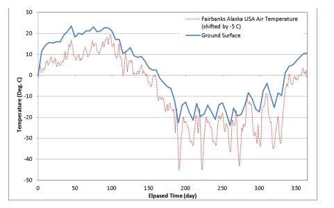
Figure 1. Ground temperature response for year 1.
Figure 2 presents the temperature decay for three elevations located at the line of symmetry beneath the thermosyphon. The results suggest that a repeatable temperature cycle is establishing at these locations after approximately two-years, which implies that the influence of the rather arbitrary starting condition is beginning to diminish. However, the downward trend of the peaks demonstrates that the analysis should be solved for additional time. The temperature at about 4.5 m below ground (green line) declines smoothly until the thermosyphons become active (Figure 3). Then, the temperature continues to decline, but in a slightly more erratic manner as the thermosyphon flux rate changes from step to step due to changing climate conditions. Once the air temperature exceeds – 0.5C, the thermosyphons become inactive (Figure 3).
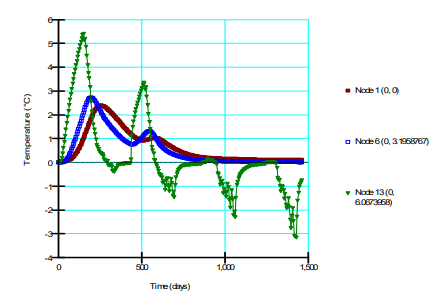
Figure 2. Temperature response at depths of 4.5 m, 7.5m, and 10.5 below ground.
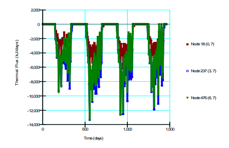
Figure 3. Heat flow (Q) from thermosyphons.
Figure 4 presents a horizontal temperature profile at an elevation of 4 m on day 1280 and 1460. Given that the climate data is commensurate with a May 1st start date, this corresponds to the beginning of July and December, respectively. The main objective of the analysis is to ensure that the thermosyphons remove the heat added by the building and that the permafrost does not suffer permanent damage below the building. The temperatures remain near or below freezing throughout the year, although the analysis should likely be solved for a longer time period.
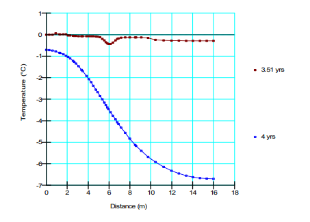
Figure 4. Temperature at a depth of 4 m.
A profile of ground temperature along the line of symmetry is presented in Figure 5. The large negative spike in temperature occurs when the thermosyphon is active and large amounts of energy are extracted from the domain. The temperature at the base of the model is at or near zero degrees by the end of the four year cycle, as shown Figure 2. The fact that the ground is not entirely frozen is due in part to the arbitrary selection of initial conditions and the deep geothermal heat flux boundary condition.
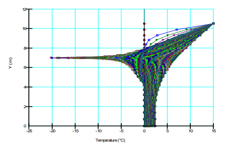
Figure 5. Temperature profile along left edge of model domain.
Summary and Conclusions
This example demonstrates the use of thermosyphons to maintain the permafrost zone beneath a heated building. The thermosyphons are modeled in end view by applying the boundary condition to a geometric point. As such, it is necessary to define the surface perimeter such that TEMP/W can convert a flux rate (q) into a flow rate (Q). The analysis also demonstrates the use of a surface energy balance boundary condition, which determines the ground heat flux based on a surface energy balance. The initial temperature of the domain is arbitrarily set to zero degrees and the analysis is solved for a number of years until a repeatable temperature cycle is established.
References
Haynes, F.D., and Zarling, J.P. 1988. Thermosyphons and foundation design in cold regions. Cold Regions Science and Technology, 15(3), 251-259.