


Introduction
The volumetric water content function, also known as the soil-water characteristic curve or water retention curve, can be determined using various laboratory methods. If the material requires a high suction for determination of this curve, a laboratory apparatus such as a Tempe cell or flow cell is typically used. The objective of this example is to illustrate the ability of SEEP/W and AIR/W to simulate the results of a Tempe cell laboratory analysis.
Background
Measuring high suctions in soils is complicated by the fact that water cavitates at negative pressures around atmosphere (about 100 kPa). One way of overcoming this problem is by elevating the air pressure in the sample and then letting the water content to reach a new equilibrium. This has the effect of translating the reference axis or reference point.
Soil suction is defined by the stress-state variable ( u/a – u/w) where is the pore-air pressure and 𝑢/w is the pore-water pressure. Consider, for example, that𝑢/𝑤 is -150 kPa and is zero (atmospheric).
The suction (𝜓) can then be calculated as:
𝜓 = (0 ‒ ( ‒ 150)) = 150 𝑘𝑃𝑎 (Equation 1)
Now consider that the air pressure u/a has been increased to 200 kPa. This value increases from 0.0 to +200 kPa and changes the pore-water pressure u/a from -150 to +50 kPa. The suction then becomes:
𝜓 = (200 ‒ ( + 50)) = 150 𝑘𝑃𝑎 (Equation 2)
The suction remains the same even though the pore-water pressure has shifted from -150 to +50 kPa. Applying the air pressure simply has altered the reference point or shifted the axis. This phenomenon can be used to devise instruments to measure suctions at high negative pore-water pressures.
One such apparatus is known as a Tempe cell. Figure 1 pictures such a cell manufactured by Soil Measurement Systems (https://www.soilmeasurement.com/tempe.html). Other manufactures are companies like Soil Moisture Equipment Corp. (https://www.soilmoisture.com).
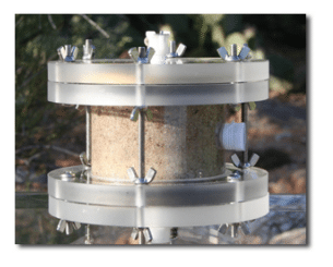
Figure 1. Tempe cell by Soil Measurement Systems (https://www.soilmeasurement.com/tempe.html).
Fundamentally, the air pressure in the cell is increased incrementally and the moisture content is allowed to come to equilibrium at each pressure level. Weighing the apparatus at each equilibrium point makes it possible to calculate the water content. This information together with the implied suction from the known air pressure makes it possible to define a soil-water characteristic curve or a volumetric water content function.
A schematic of the apparatus is given in Figure 2. The soil sample sits on what is known as a high air-entry disk. Water can pass through the disk but the air cannot if the air pressure is below the air-entry value.
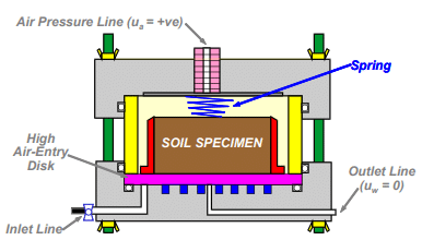
Figure 2. Schematic of a Tempe cell.
The chamber is pressurized and then the water content is allowed to come to equilibrium. Then the air pressure is increased and the process is repeated. Often the sample is prepared as a slurry and then allowed to consolidate under a nominal load before applying the air pressure. So the testing starts with 100% degree of saturation at, in essence, zero pore-water pressure and zero pore-air-pressure; that is, the suction is zero at the start of the test.
Numerical Simulation
Figure 3 shows the numerical configuration for the example. The sample is considered to be 60 mm in diameter and 30 mm thick. Only half of the sample needs to be included in the analysis due to the symmetry about the central axis, which lends itself to an axisymmetric type of analysis. The full sample was simulated by using the axisymmetric analysis type with the full 360° for the central angle settings (Figure 4).
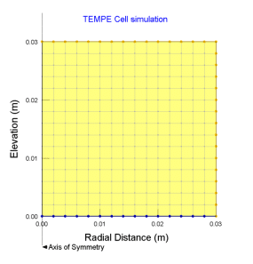
Figure 3. Problem configuration.
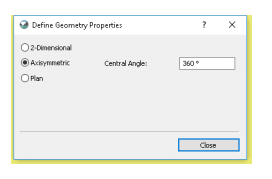
Figure 4. Axisymmetric settings for analysis of pseudo-3D sample.
There are a total of six analyses in the Project (Figure 5). The air pressure in the Tempe cell is incrementally increased in each of the transient analyses. Numerically, this means that each pore-air pressure increase builds on the previous equilibrium condition; that is, previous analyses results.
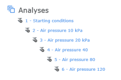
Figure 5. Analysis Tree for the Project.
The initial analysis (1 – Starting conditions) is a steady-state water transfer analysis with the air transfer processes activated (Figure 6). This analysis acts as the initial conditions for the remaining transient analyses in the Analysis Tree. The remaining transient analyses also have the air and water transfer processes activated, with each subsequent analysis acting as a child to the previous analysis.
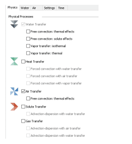
Figure 6. Physics tab for the water and air transfer processes.
The sample is considered to be a silty soil with a porosity of 0.45. The saturated/unsaturated material mode was used to define the hydraulic properties of the soil. The volumetric water content was estimated using the internal silt sample type with a saturated volumetric water content of 0.45 (Figure 7). The hydraulic conductivity function was estimated using the volumetric water content curve with a saturated hydraulic conductivity of 1 x 10⁻⁴ m/s (Figure 8).
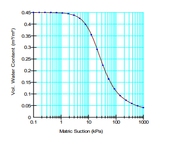
Figure 7. Volumetric water content function of the silty sample.
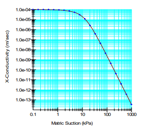
Figure 8. Hydraulic conductivity function of the silty sample.
The air conductivity is a function of the water content. When the soil is saturated, virtually no air can pass through the sample. Air can, however, pass quite freely through the soil when the sample is dry. For this example, the dual phase air material model was used to ensure that an air conductivity function can be defined to accurately simulate both the air and water processes.
The air conductivity can be estimated from the volumetric water content function above, together with a specified dry-soil conductivity. The dry air conductivity is specified as 1.0 m/s. The resulting estimated function is shown in Figure 9.
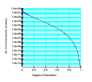
Figure 9. Air conductivity function.
The hydraulic conditions were defined in all of the analyses using a zero pressure head boundary condition along the bottom of the soil sample. This boundary condition simulates the conditions of the high AEV porous stone allowing water to drain from the sample as the air pressure increases. The initial air conditions were defined using a zero pressure (or relative atmospheric pressure) boundary condition along the top and right boundaries of the sample. No boundary conditions were applied to the left boundary, as this is considered the axis of symmetry in the axisymmetric analysis.
As the air pressure increases in the Tempe cell, the air boundary conditions change to accommodate this air pressure change. For example, the first transient analysis simulates an increase in the air pressure by 10 kPa. Both the air pressure applied and the duration of each subsequent analyses increase until a total air pressure of 120 kPa is applied to the soil sample and a total duration of 5.22 hours is reached. The global element size was set to 2 mm for the entire sample domain.
Results and Discussion
The first three transient analyses simulated the increase in air pressure from the initial 0 kPa to 10 kPa, 20 kPa and 40 kPa. The resulting pore-water pressure and volumetric water content profiles for a point chosen along the centre axis at an elevation of 16 mm are shown in Figure 10 and Figure 11, respectively.
Notice how the volumetric water content is, in essence, constant for a few seconds at the start. This is the situation until the sample begins to de-saturate. As the suction increases, the water content decreases once air starts entering the sample. As higher increments of applied air pressure are used, the time to reach equilibrium in the pore-water pressure and water content increase.
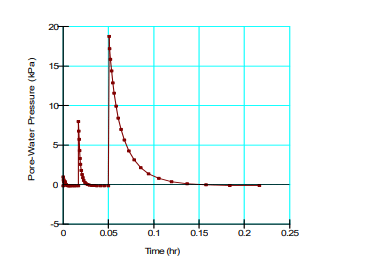
Figure 10. Pore-water pressure profile after the first 3 increases in air pressure (10 kPa, 20 kPa and 40 kPa).
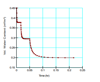
Figure 11. Volumetric water content profile after the first 3 increases in air pressure (10 kPa, 20 kPa and 40 kPa).
Figure 12 and Figure 13 show the pore-water pressure and volumetric water content profile for the same node after the final 2 air pressure increments are applied to the sample. Again, the time required to reach equilibrium continues to increase as the air pressure increases. Initially, when the air pressure is applied, the pore-water pressure spikes near saturation, until the water content decreases and equilibrates.
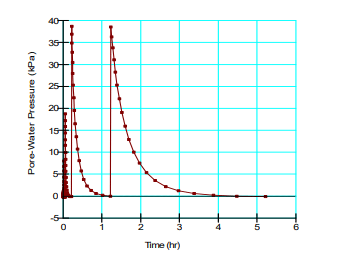
Figure 12. Pore-water pressure profile after the last 2 increases in air pressure (80 kPa and 120 kPa).
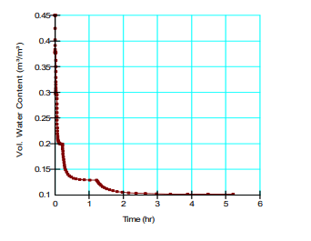
Figure 13. Volumetric water content profile after last 2 increases in air pressure (80 and 120 kPa).
At the end of the test, the volumetric water content is approximately 0.1 at a matric suction of 120 kPa. This falls exactly on the specified VWC function shown in Figure 7.
Summary and Conclusions
This simulation does not have much practical application. It does, however, clearly illustrate the physical process which is enlightening in itself. For example, it demonstrates that early on, when the sample is near saturation, the equilibrating process is very fast. Later, as the sample becomes drier and the air pressure increases, the equilibrating process is much slower. This is primarily due to fact the hydraulic conductivity diminishes rapidly as the soil de-saturates.
Moreover, this illustrative example demonstrates that the coupled SEEP/W and AIR/W products can handle problems that involve pore-air pressure changes and the corresponding air flow.