Technical Tuesday: Using Leapfrog Edge for dynamics grade control in underground mines

This workshop will cover:

• Tips and tricks for generating underground workflows in Leapfrog Edge
• Fundamental steps required to set up an estimation domain
• Evaluating information onto our Block Models
• Data preparation and processing techniques including variography
• Summary of depletion modelling and stope reporting

Video Transcript

[00:00:00.000](gentle music)

[00:00:10.440]<v Steve>Thank you for taking the time today</v>

[00:00:11.900]to listen to this webinar.

[00:00:14.100]My name is Steve Law,

[00:00:15.410]and I’ve been a senior project geologists

[00:00:17.480]with Seequent for the past two and a half years.

[00:00:21.100]I am the Technical Lead for Leapfrog Edge,

[00:00:23.800]my background is primarily as a senior geologist

[00:00:26.630]in Production and Resource geology roles.

[00:00:30.980]I will be presenting an example workflow

[00:00:33.550]of how to use Seequent’s mining solution software

[00:00:36.940]to enhance the grade control process

[00:00:39.320]in an underground operating environment.

[00:00:42.110]Most aspects could also be utilized

[00:00:44.250]in an open-cut operation as well.

[00:00:48.170]The key point of today’s demonstration

[00:00:50.470]is to show the dynamic linkages

[00:00:52.190]between Leapfrog Geo and Leapfrog Edge,

[00:00:54.810]managed within the framework of Seequent Central.

[00:00:58.610]I will briefly touch on data preparation

[00:01:00.810]and an example workflow, splitting projects by discipline.

[00:01:05.380]While it’s not designed as a training session,

[00:01:07.800]I will cover the basic domain centric setup within Edge,

[00:01:11.090]and show the different components, including variography.

[00:01:14.770]I will focus a little more on the block model setup

[00:01:17.340]and how to validate the grade-control model

[00:01:20.020]and report results, as this part of the workflow

[00:01:22.880]is a little different to how you may be used to doing it.

[00:01:27.130]The Seequent Solution

[00:01:28.290]encompasses a range of software products

[00:01:30.770]applicable for use across the mining-value chain.

[00:01:34.580]Today, I’ll focused on Seequent Central,

[00:01:36.810]Leapfrog Geo and Leapfrog Edge,

[00:01:39.320]which integrated together, present the opportunity

[00:01:41.760]to deliver key messages to different stakeholders.

[00:01:45.320]Leapfrog Geo remains the main driver, but I will show

[00:01:48.590]how, by utilizing the benefits of Edge and Central,

[00:01:52.050]the workflow in an underground grade-control environment

[00:01:55.120]can be enhanced.

[00:01:58.260]Grade control is the process of maximizing value

[00:02:01.030]and reducing risk.

[00:02:02.800]It requires the delivery of tons in an optimum grade

[00:02:06.000]to the mill, via the accurate definition of ore and waste.

[00:02:10.170]It essentially comprises data collection,

[00:02:12.850]integration and interpretation, local-resource estimation,

[00:02:17.730]stope design, supervision of mining,

[00:02:19.610]and stockpile management and reconciliation.

[00:02:24.530]The demonstration today will take us up to the point

[00:02:27.300]where the model would be passed on

[00:02:28.700]to mine planning and scheduling.

[00:02:32.300]The foundation of all grade control programs

[00:02:34.830]should be that of geological understanding.

[00:02:37.910]Variations require close knowledge of the geology

[00:02:42.350]to ensure optimum grade, minimal dilution,

[00:02:45.210]and maximum mining recovery.

[00:02:48.050]By applying geological knowledge,

[00:02:50.170]the mining process can be both efficient and cost effective.

[00:02:55.270]The integration and dynamic linkage of the geology

[00:02:57.920]with the Grade Control Resource Estimate

[00:03:00.160]leads to time efficiencies.

[00:03:02.870]We can reduce risk

[00:03:04.500]with better communication via the Central Interface,

[00:03:07.830]which offers a single source of truth

[00:03:09.660]with full version control,

[00:03:11.520]member permissions and trackability.

[00:03:15.170]Better decisions are achievable, as teams work together

[00:03:18.510]to collaborate on the same data and models.

[00:03:21.690]Everyone can discuss and explore

[00:03:23.300]different geological interpretations

[00:03:25.330]and share detailed history of the models.

[00:03:28.920]Central provides a quality framework for quality assurance,

[00:03:34.000]as an auditable record and timeline of all project revisions

[00:03:37.530]is maintained.

[00:03:39.080]For those of you

[00:03:39.913]who have not been exposed to Seequent Central,

[00:03:42.050]here is a brief outline.

[00:03:44.030]It is a server-based project management system

[00:03:46.860]with three gateways for different users and management.

[00:03:50.740]The Central portal is where administrators

[00:03:53.720]can assign permissions for projects stored on the server.

[00:03:57.980]Users will only see the projects

[00:03:59.610]they have permission to view or edit.

[00:04:02.940]The Central Browser allows users to view and compare

[00:04:06.310]any version of the Leapfrog Project

[00:04:08.190]within the store timeline.

[00:04:10.290]The models cannot be edited,

[00:04:11.800]but output messages can be shared

[00:04:14.170]with users who do not require direct access to Leapfrog Geo.

[00:04:18.450]There is also a data-room functionality,

[00:04:21.270]which equates to a Dropbox-type function

[00:04:23.600]assigned to each project.

[00:04:26.520]Today, I will focus on the Leapfrog Geo Connector,

[00:04:29.660]which is where we can define various workflow structures.

[00:04:32.910]Specifically, we will focus

[00:04:34.790]on one where the projects are split

[00:04:36.870]according to geology modeling or estimation functions.

[00:04:42.260]The following demonstration will show the workflow

[00:04:44.840]for an underground dynamic system,

[00:04:47.530]using Leapfrog Geo software.

[00:04:49.860]We are going to use the Central Interface,

[00:04:52.510]and this involves having a central Cloud server

[00:04:55.210]wherein projects are stored, and we then access the project

[00:04:59.310]directly from within Leapfrog Geo itself.

[00:05:04.510]I have a project set up here,

[00:05:07.010]which has been set up with three separate branches,

[00:05:09.380]a geology branch, an estimation branch,

[00:05:13.000]and an engineering branch.

[00:05:14.890]I’ll primarily be focusing on

[00:05:16.660]the geology and estimation branches.

[00:05:20.670]The way Central works

[00:05:21.630]is that you store your individual projects on a server,

[00:05:25.590]and each iteration of the project is saved in this timeline.

[00:05:30.140]So the most recent project

[00:05:32.080]is always the one at the top of the branch.

[00:05:35.070]So, if we’re looking at geology branch,

[00:05:37.220]here you can see geology, we go to the top level of geology,

[00:05:41.580]and then this is the latest geology project.

[00:05:44.830]Again, for estimation, we followed through

[00:05:47.900]until we find the top-most branch.

[00:05:50.390]And this is the top most and most recent resource estimate.

[00:05:55.320]To work with Central, we download the projects

[00:05:58.820]by right-clicking on the required branch,

[00:06:01.530]and they are then local copies.

[00:06:03.900]So in this instance,

[00:06:05.090]I have four local copies stored on my computer.

[00:06:08.280]I am no longer connected to the Cloud server

[00:06:11.100]for working on these, I can go offline, et cetera.

[00:06:14.950]The little numbers, 1, 2, 3, and 4,

[00:06:17.800]refer to the instances up here, so I always know

[00:06:21.080]which project I’m working on at any one time.

[00:06:24.700]For this demonstration, I’m going to start off

[00:06:27.510]with the geology model set up as a pre mining resource,

[00:06:31.780]so down here at Project 1.

[00:06:42.750]So the data set we’re working with here

[00:06:45.260]is a series of surface drill holes,

[00:06:47.340]diamond drill holes, primarily.

[00:06:49.220]And it is basically a vein system.

[00:06:53.950]And I have set up a simple series of four veins

[00:06:58.663]as part of a vein system.

[00:07:06.900]The main vein is Vein 1, and then we have Veins 2, 3, and 4,

[00:07:11.470]coming off it as splice.

[00:07:15.810]This model has been set up in a standard way,

[00:07:18.290]so we had the geological model.

[00:07:20.110]And we’re going to use this

[00:07:21.910]as the basis for doing an estimate on Veins 1, 2, 3, and 4.

[00:07:29.350]If you did not have Central, then the block model

[00:07:31.460]would need to be created within this project,

[00:07:34.000]under the Block Models and Using the Estimation Folder.

[00:07:37.730]And then if you were going to update,

[00:07:40.610]you would potentially freeze the block model

[00:07:43.300]by using the new Freeze/Unfreeze function.

[00:07:46.870]And then whilst we’re updating the geological model,

[00:07:49.650]the block model won’t change until we unfreeze it.

[00:07:53.320]The problem with this is that we don’t ever have a record

[00:07:57.510]of what the previous model looked like,

[00:07:59.050]unless we zipped the project

[00:08:00.840]and dated it and stored it somewhere.

[00:08:04.180]The advantage of Central is that each iteration is stored

[00:08:09.560]so that we can always go back

[00:08:10.960]and see what the model looked like beforehand.

[00:08:14.600]So the geology model has been set up,

[00:08:17.010]I’m going to go now into the first estimation project,

[00:08:22.540]where I set up the pre mining resource.

[00:08:24.560]So in this case, this is Local Copy 2,

[00:08:27.340]and the branch is Estimation.

[00:08:39.370]The key difference here when using Central

[00:08:41.590]is that rather than directly linking

[00:08:43.860]to a geological model within the project,

[00:08:46.570]the domains are coming from centrally linked meshes.

[00:08:50.220]So under the Meshes folder,

[00:08:52.000]you can see we have these little, blue mesh symbols.

[00:08:55.530]And if I right-click on these, it’s reload latest on branch,

[00:09:00.640]or from the project history.

[00:09:02.760]The little clock is telling me

[00:09:04.140]that since the last time I opened up this project,

[00:09:08.010]some thing has changed in the underlined geological model.

[00:09:12.070]Once we go reload latest on project,

[00:09:14.890]then the little clock will disappear.

[00:09:18.210]So all the meshes that I’m using within the estimation

[00:09:21.870]are accessing directly from centrally-linked meshes.

[00:09:27.230]I’m just going to focus now on a quick run through

[00:09:30.560]of how to set up a domain estimation in Edge using Vein 1.

[00:09:35.860]Edge works on a domain-by-domain basis.

[00:09:39.370]And we work on one domain and one element,

[00:09:41.580]and then we can copy and keep going through

[00:09:44.330]until we create all four or more.

[00:09:48.200]Each estimation is its own little folder.

[00:09:51.360]So we have here AU_PPM Vein 1,

[00:09:56.410]and we have, within that, a series of sub-folders.

[00:10:00.030]We can check quickly what the domain is, to make sure

[00:10:03.240]that we’re working in the space that we expect to be,

[00:10:06.500]and the values shows us the composites,

[00:10:12.520]but it’s the midpoints of the intervals.

[00:10:14.570]So it’s been reduced to point data,

[00:10:17.660]which we can still display as normal drill holes,

[00:10:21.580]and we can do statistics on that

[00:10:24.160]and have a look at a histogram, et cetera,

[00:10:28.180]log probability plots.

[00:10:35.670]There is also a normal score functionality,

[00:10:39.230]particularly when working

[00:10:40.660]with gold data sets that are quite skewed,

[00:10:43.440]we may wish to transform the values to normal scores.

[00:10:46.770]So to do that, we would right-click on the values,

[00:10:50.510]and there would be a transformed values function,

[00:10:54.160]if it hasn’t been run already as it has been here.

[00:10:57.130]So that produces a normal scores,

[00:11:00.150]which is purely changing the data to a normal distribution.

[00:11:04.710]And it decreases the influence of the high values,

[00:11:09.160]whilst the variogram is being calculated.

[00:11:11.960]It is then back-transformed into real space

[00:11:14.440]before the estimate is run.

[00:11:18.530]If we wish to edit our domain or our source data,

[00:11:22.230]we can always go back to opening up at this level.

[00:11:25.380]This is where we choose the domain, and we can see here

[00:11:27.810]that it’s directly linked back to the central meshes here.

[00:11:33.220]And then the numeric values can come from any numeric table

[00:11:37.220]within our projects, by the role Drill Hole Data,

[00:11:40.640]or Composited Data if we have it,

[00:11:43.200]but we have the option of compositing at this point,

[00:11:46.400]which is what I’ve chosen to do.

[00:11:47.790]The compositing done here is exactly the same

[00:11:50.530]as if the compositing is done

[00:11:52.470]within the drill-hole database, first,

[00:11:55.380]it just depends on some processes

[00:11:57.210]or whether it needs to be done there or here.

[00:12:02.450]Variography done

[00:12:03.283]is all done within the Special Models folder.

[00:12:06.110]In this instance, I’ve done a transformed variogram

[00:12:08.840]on the transform values because it gives a better result.

[00:12:15.930]The way we treat variography

[00:12:17.210]is not too dissimilar to other software packages,

[00:12:20.180]we’re still modeling into three prime directions

[00:12:23.560]relative to our plan of continuity.

[00:12:26.970]The radio plot is within our plane,

[00:12:29.980]so in this case it’s set along the direction of the vein,

[00:12:33.320]and then we’re changing the red arrow,

[00:12:36.190]it’s changing pitching plans.

[00:12:38.770]The key thing when using Leapfrog is that the variogram

[00:12:42.260]is always linked through to the 3D scene,

[00:12:47.050]so if we move anything within the forms,

[00:12:52.100]then the ellipse itself will be changing in the 3D scene,

[00:12:56.250]and vice versa, we can move the ellipse

[00:12:58.630]and it will change the graphs in this side as well.

[00:13:06.350]This is a Normal Scores 1.

[00:13:08.500]So once the modeling has been done

[00:13:10.840]and we can manually change using the little leavers

[00:13:13.940]or by just typing in the results through here, and hit Save.

[00:13:18.340]We do need to use the back transform,

[00:13:20.600]so that will process it,

[00:13:23.020]so that it’s ready to use directly in the estimate.

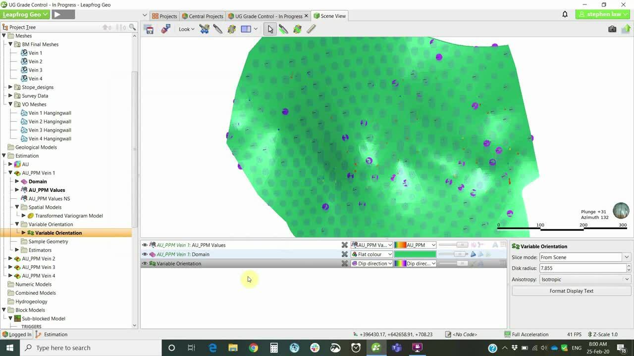
[00:13:30.740]Another good feature that we have within Edge

[00:13:33.150]is the possibility of using variable orientation,

[00:13:36.350]which is a defectively dynamic anastrophe.

[00:13:40.021]So locally takes into account

[00:13:42.350]local changes in the underlying domain’s geometry.

[00:13:48.570]We can use any open mesh to set this up.

[00:13:53.310]In this case, I’m using a vein hanging-wall surface

[00:13:56.680]to develop this.

[00:13:59.950]Again, these surfaces

[00:14:01.510]have been imported directly from the geology model

[00:14:05.270]as centrally linked meshes.

[00:14:07.080]So as the geology model changes,

[00:14:08.910]these will also be able to be updated if necessary.

[00:14:14.110]There was a visualization of the variable orientation,

[00:14:19.100]and that is in the form of these small disks,

[00:14:23.140]which you can define on a grid

[00:14:25.710]and you can display dip direction or Dip.

[00:14:30.390]And if we have a look in a section,

[00:14:36.320]we can get an idea of how the ellipsoid will change.

[00:14:40.610]So in this way, the variogram ellipse will move through

[00:14:44.290]and change its orientation relative to the local geometry,

[00:14:47.770]rather than having to be set

[00:14:49.290]at that more averaged orientation across the whole vein.

[00:14:55.820]Sample Geometry is a couple of declustering too,

[00:14:59.460]which I will not go into at this stage.

[00:15:02.300]The key folder that we need to work with

[00:15:04.750]is the Estimates folder,

[00:15:06.700]and this is where we can set up either inverse distance,

[00:15:09.960]nearest neighbor, ordinary or simple kriging,

[00:15:12.970]or RBF estimated the same type of algorithm that we use

[00:15:16.900]under our geological modeling and numeric models.

[00:15:20.656]In this instance, I’ve set up two passes for the kriging,

[00:15:24.770]so I can open up both of those at the same time.

[00:15:32.490]We can set top cutting at this level.

[00:15:34.990]So in this case, I’ve top cut to 50.

[00:15:37.760]We don’t have to do it there

[00:15:39.880]if we can’t, we could do it in the composite file earlier,

[00:15:43.150]but it wouldn’t need to be done outside of Leapfrog first.

[00:15:46.570]The interpolant tells peaks

[00:15:48.210]whether it’s ordinary kriging or simple kriging,

[00:15:50.900]and we define the discretization,

[00:15:53.170]which is based on the parent block.

[00:15:55.450]So this is dividing the parent block that dimension,

[00:15:58.250]into four by four by four.

[00:16:01.570]We picked the variogram model,

[00:16:03.390]so it was only one to choose from.

[00:16:05.630]The estimates can only see the variograms

[00:16:08.460]that are sitting within

[00:16:09.810]the particular folder that you’re working from.

[00:16:12.740]But you can have as many different variogram models

[00:16:14.870]as you like, to choose from and test different parameters.

[00:16:19.690]The ellipsoid, so when we first developed this,

[00:16:23.210]it is usually set to the variogram,

[00:16:26.690]and then in this case we are overriding it

[00:16:29.580]by using the variable orientation.

[00:16:31.970]So it maintains the ranges, but changes the orientation,

[00:16:36.347]relative to the mesh.

[00:16:39.630]You can see here that the second search that I’ve set up

[00:16:42.580]is simply double the ranges of the first.

[00:16:47.300]We have a series of

[00:16:49.350]fairly-standard search criteria and restrictions,

[00:16:52.650]so minimum/maximum number of samples, outlier restriction,

[00:16:56.360]which is a form of top-cutting but not quite as severe.

[00:16:59.620]So you’re only top-cutting

[00:17:01.270]high values beyond a certain distance,

[00:17:04.220]sector search as both Oakton or quadrant,

[00:17:07.390]and drill-hole limit,

[00:17:08.640]which is maximum number of samples per drill hole.

[00:17:12.100]In this case, I’m telling this effectively says

[00:17:15.500]that I must have at least one drill hole to proceed.

[00:17:19.850]The second search is looking at a greater distance,

[00:17:22.820]reducing down to number one sample and no restrictions.

[00:17:26.170]And this is simply to try and get a value

[00:17:28.640]inside all the blocks,

[00:17:30.110]which is needed for reporting later on.

[00:17:33.550]One point of difference for Edge compared to other software

[00:17:36.650]is how we define variables.

[00:17:39.010]So the grade variable name is this name down here,

[00:17:42.640]which is automatically assigned, but can be changed.

[00:17:45.850]Then rather than having to set up variables

[00:17:48.080]within a block-model definition, we simply tick the boxes

[00:17:51.440]for the ones that we may want to store.

[00:17:53.570]So if we want to store kriging variance,

[00:17:55.450]we’d simply tick the box here.

[00:17:57.980]It doesn’t matter if you don’t tick it individually

[00:18:00.390]and decide you need it later,

[00:18:01.660]you can always come back to here

[00:18:03.230]and tick the boxes as necessary.

[00:18:05.800]I find that it is useful not to tick them

[00:18:08.520]if you don’t need them,

[00:18:10.130]’cause it makes the processes quite busy later on.

[00:18:14.720]So let us set up the parameters.

[00:18:17.240]So Estimation folder can be thought of as a parameter file.

[00:18:23.360]And this is where we set up all the parameters

[00:18:25.120]for our estimate.

[00:18:26.600]One key concept that we need to understand

[00:18:29.670]is the concept of a combined estimator.

[00:18:33.660]If I evaluate or view these runs, Run 1 and Run 2,

[00:18:38.280]in the block model, I’ll only be able to display

[00:18:41.030]either Run 1 or Run 2 at a time,

[00:18:44.610]as well as I’ve got four veins set up,

[00:18:47.800]I can only see each vein individually.

[00:18:50.540]So I need to combine them together to be able to view

[00:18:54.090]the whole gold grade of everything at once.

[00:18:57.520]And this is done by creating a new combined estimator,

[00:19:00.770]which is simply like a merge table

[00:19:02.960]from the geological database.

[00:19:05.440]So in this instance, I’ve set up all of the veins,

[00:19:09.770]the veins, and each pass for each.

[00:19:11.900]The order of the domains isn’t critical

[00:19:14.610]because they’re all independent of each other,

[00:19:17.270]but the order of the passes is very important.

[00:19:20.510]So Pass 1 must be on top, higher priority,

[00:19:24.640]and then that means that that is looked at first,

[00:19:28.220]then any blocks that do not have a value in them after that

[00:19:31.130]is run, we’ll then use the Pass 2 parameters.

[00:19:34.770]If we inadvertently place Pass 2 above,

[00:19:38.040]then it effectively overrides past one.

[00:19:42.000]It is re-estimating every block with Pass 2 parameters

[00:19:46.130]as it does it, so the order is quite important.

[00:19:51.510]As you add new domains, then you can simply select,

[00:19:55.830]that’ll be available over here on the left,

[00:19:58.550]and you can move them across at will.

[00:20:04.290]This is often the variable that is exported

[00:20:06.870]to other software packages in a block model,

[00:20:09.240]so I tend to try and keep the naming of these

[00:20:11.300]quite short and simple, because a lot of packages

[00:20:14.130]are limited to how many characters they can accept.

[00:20:17.370]Again, outputs can be calculated for the combined estimate,

[00:20:21.190]so we can store any of these,

[00:20:22.980]and it does automatically assign an estimator number,

[00:20:27.080]and a domain number.

[00:20:29.070]So if we have two passes, then it will slightly code

[00:20:33.160]the passes slightly different shades.

[00:20:35.890]In this instance, Pass 1 and 2,

[00:20:38.410]slightly different grades of Aqua.

[00:20:42.790]Since we have all our estimates

[00:20:44.280]and combined estimates set up,

[00:20:46.300]we then proceed to setting up a block model.

[00:20:49.110]And this is where we view, validate and report.

[00:20:52.390]Validation Swath plots, and the resource reports

[00:20:57.390]are all embedded within the block model,

[00:20:59.970]so when the block model updates,

[00:21:01.810]these ancillary functions update as well.

[00:21:08.220]In this case, we’re using a sub-block model,

[00:21:10.550]we can do regular models, which is simply a new block model.

[00:21:13.800]It’s exactly the same, except for a Sub-block model,

[00:21:17.730]we have sub-block count,

[00:21:19.500]which is the parent block size divided by the count.

[00:21:22.130]So in this case, we’ve got 10-meters parent blocks,

[00:21:25.510]and two-meter sub-blocks, in all directions.

[00:21:29.360]Sub-block models can be rotated in both deep and estimate.

[00:21:33.180]Sub-blocking triggers is important.

[00:21:35.850]So for us, we are bringing across the meshes of each vein.

[00:21:40.640]So if we add a new vein, we would need to bring that

[00:21:43.910]across to the right-hand side.

[00:21:46.300]And then the most important tab is the Evaluations tab.

[00:21:50.640]Anything that we want to see in the block model or run,

[00:21:54.183]needs to come across to the right-hand side.

[00:21:57.240]So in this case, we are running the kriging for Pass 1

[00:22:02.440]in each of the veins, and I’ve got the combined estimator.

[00:22:05.980]Now, I do not need to bring across the individual components

[00:22:09.920]if I have a combined estimator,

[00:22:11.980]it’s just that I want to look at the underlying composites

[00:22:16.540]against the estimate in a Swath plot,

[00:22:18.720]I can only do so with the underlying individual run files,

[00:22:23.420]not the combined estimator.

[00:22:26.220]So for validation, I do need the individuals,

[00:22:30.030]and normally I would just look at Pass 1,

[00:22:32.360]but if I’m just reporting, I don’t need these,

[00:22:35.200]and I can remove them and take them across to the left,

[00:22:38.300]and would just have the combined estimators.

[00:22:42.040]So whenever a new parameter is set up

[00:22:44.540]in the Estimation folder,

[00:22:46.230]then you must go to the corresponding block model

[00:22:49.080]and move it across to the right on the evaluation tab

[00:22:53.230]for it to run.

[00:22:56.340]To visualize our results,

[00:23:00.640]we have got all of the evaluations that we told it to use,

[00:23:05.400]this is our combined estimator,

[00:23:07.430]so we can see the results of all four veins.

[00:23:20.670]And there are some other tools here, against each parameter,

[00:23:25.830]we’ve got this status.

[00:23:27.350]So if we have a look at Vein 1 by itself,

[00:23:30.560]so that just shows the results for Vein 1.

[00:23:34.500]And we can look at the status, and this shows us

[00:23:41.000]which blocks we estimated and which are not.

[00:23:43.310]So we still have a few blocks around the edges

[00:23:46.200]or away from data, that aren’t estimating at this stage.

[00:23:51.220]Anything that we stored in the outputs volume,

[00:23:54.120]so their number of samples can be displayed.

[00:23:57.320]So we can see here

[00:23:58.290]that we’ve got plenty of samples in the middle,

[00:24:00.520]but it gets quite sparse around the edges.

[00:24:07.400]Another feature of block models is Calculations And Filters.

[00:24:12.000]So what this one is doing

[00:24:13.910]is we store all the possible variables

[00:24:17.490]that we may use within the calculation.

[00:24:20.100]And in this one, I’ve made a new numeric calculation,

[00:24:24.300]which says, “If there is a grade in the block,

[00:24:28.370]then use that grade, but if there is not, make it 0.001.”

[00:24:32.960]So this is just one way of trying to remove

[00:24:35.940]blocks that have not been estimated, the other way would be,

[00:24:40.362]could set up a nearest neighbor with a large search,

[00:24:44.590]and append that to the combined estimator at the very end.

[00:24:49.550]So multiple ways of dealing with sparse blocks.

[00:24:54.170]In this case, a calculation

[00:24:56.180]can be viewed in the block model.

[00:24:58.680]Variables are parameters that can be used in a calculation,

[00:25:02.340]such as something like gold price,

[00:25:04.450]but you can’t visualize it in the model.

[00:25:07.550]And then filters are simply query filters

[00:25:10.000]to find as we would in drill hole,

[00:25:11.990]but it’s applying to the actual block model.

[00:25:15.610]So I’ve created this gold final calculation,

[00:25:21.930]and it can be displayed, because it shows up down in here.

[00:25:31.100]And we can see all our grades above two grams.

[00:25:37.132]So that’s the basic setup of the very-first resource model.

[00:25:42.210]So coming back to here, we would then be ready to…

[00:25:45.670]We have some new grade-control drilling,

[00:25:48.140]so we’d go to the geological model

[00:25:50.770]where that drilling was upended, which is number three.

[00:26:02.740]So we have

[00:26:03.863]a series of drill-hole, grade-control, infill holes

[00:26:07.230]that have been drilled as a fan from underground.

[00:26:21.420]Whoever’s in charge of working on the interpretation,

[00:26:29.820]will go through each of the drill holes, new drill holes,

[00:26:32.910]and using the tool selection that had already been set up,

[00:26:37.100]could reassign

[00:26:38.230]according to which vein things are related to,

[00:26:40.990]and then the model will update.

[00:26:45.460]One handy thing to do is we are linking meshes directly,

[00:26:49.710]but we can’t link drill-hole information at the moment.

[00:26:52.810]So what I would often do at this stage is export

[00:26:55.840]all of the information from the drill hole data set.

[00:26:59.830]I could then load it to

[00:27:03.270]the data room associated with this particular project.

[00:27:14.100]So each project in the portal has a files folder,

[00:27:18.980]and within this folder, which works similar to a Dropbox,

[00:27:23.230]you could put the current drill-hole-database files,

[00:27:27.290]and then we could download those,

[00:27:29.750]and they will be ready to import into our Estimation folder.

[00:27:33.770]This portal is also where we can assign users

[00:27:37.200]to the project,

[00:27:39.857]and each project can have its own specific users.

[00:27:46.110]So we go back to this one and have a look at the users.

[00:27:57.292]I can see that we’ve got five users,

[00:28:00.480]and they are all editors.

[00:28:02.720]You can have people who only are going to be able to view

[00:28:06.639]a few of the project,

[00:28:07.500]and they would use Central Browser to do that,

[00:28:09.350]but they cannot edit anything.

[00:28:14.432]We have updated the geology, so we go back to our estimation

[00:28:23.330]and we would open that up, and reload the new drilling.

[00:28:31.090]So we have two options, if it’s brand new drilling

[00:28:33.550]that doesn’t exist anywhere in the project,

[00:28:35.930]then we could use the Append function,

[00:28:39.180]so appending the drill holes.

[00:28:40.970]If you’re accessing a main database

[00:28:44.870]and everything’s added to that, then you could reload,

[00:28:47.860]and that will put in all the new holes and any changes.

[00:29:02.079]So the drill holes are updated,

[00:29:04.690]and then within the Meshes folder,

[00:29:06.890]all the veins that may have changed need to be updated.

[00:29:09.300]So we just simply go reload latest on branch,

[00:29:12.090]then the block model will then rerun,

[00:29:15.820]and we are ready to report and validate.

[00:29:21.500]Swath plots are maintained within the block model itself.

[00:29:26.360]So to start with, we can create a new Swath plot.

[00:29:31.400]Once it’s been created,

[00:29:32.590]it is stored down under Graphs And Tables,

[00:29:35.380]and then we can open it up at any time,

[00:29:38.400]and have a look at them.

[00:29:40.090]It automatically creates the X, Y, and Z directions,

[00:29:45.000]and we can add as many or few items as we like

[00:29:48.760]using the selected numeric items.

[00:29:51.240]In this case, I’m wanting to compare

[00:29:53.520]the kriging in Pass 1,

[00:29:55.240]and I want to look at their original composites.

[00:29:57.810]So to do that, I need to turn them on down here.

[00:30:03.030]So you can see that I’ve got the clips composite values

[00:30:06.510]showing in the red.

[00:30:08.790]If I had an inverse distance estimator, I could add that,

[00:30:12.920]and then I could compare the kriging

[00:30:14.190]against this inverse distance.

[00:30:18.969]We’re ready to report against our block model.

[00:30:23.630]The key to reporting within Leapfrog Edge

[00:30:26.830]is that we need to have a geological model

[00:30:31.580]with output volumes that can be evaluated.

[00:30:34.690]So at this stage, we cannot directly evaluate meshes,

[00:30:38.550]so they need to be built into a geological model.

[00:30:42.420]So in this instance, I have a GM Domain,

[00:30:45.910]which is simply taking the meshes directly, as we can see,

[00:30:50.310]using the new intrusion from Surface,

[00:30:56.300]and that builds them up.

[00:30:58.430]It’s also a good way of being able to combine domains.

[00:31:02.080]So if, for instance, we wanted to estimate Vein 2, 3, and 4,

[00:31:07.030]as a single domain, then we could basically assign

[00:31:13.320]whatever name is in the first lithology.

[00:31:15.950]So I could call this Kriging Zone 2,

[00:31:18.640]and I can still leave this as Vein 2 here,

[00:31:21.570]but I just use Kriging Zone 2

[00:31:23.670]as the first lithology for all three,

[00:31:26.370]and then my output volumes,

[00:31:27.820]I would just have Kriging Zone 2,

[00:31:30.050]and Vein 1, I could have a single vein for that one.

[00:31:34.100]So it’s a great way

[00:31:35.580]of being able to combine our domains together,

[00:31:38.330]to run estimates.

[00:31:41.600]We often use classification, and often we’ll have shapes

[00:31:44.970]maybe generated in another software,

[00:31:47.130]or we could use polylines within Leapfrog to create a shape.

[00:31:51.460]In this instance, I’ve just done a quick distance buffer

[00:31:55.440]around the drill holes, and I have referenced that,

[00:31:58.560]so then I ended up with two output volumes

[00:32:02.788]for a measured and indicated area,

[00:32:07.990]and the rest would be inferred.

[00:32:10.430]The same for any stoping panels.

[00:32:13.130]If we wish to report within shapes,

[00:32:15.610]stipe shapes or drive shapes,

[00:32:17.490]they need to be built into a geological model first.

[00:32:20.320]So in this instance, I’ve generated some panels.

[00:32:25.460]So we’ve got Panel 1, 2, 3, 4, 5.

[00:32:33.779]I needed this to be combined against mineralization shape,

[00:32:38.610]so I’ve actually used a Combined model,

[00:32:43.560]and I have the combined,

[00:32:47.850]so I have the stipe panels confined to Vein 1,

[00:32:52.310]which I will report against.

[00:32:57.620]So resource reports

[00:32:58.960]are gained built within the block model itself.

[00:33:01.460]So new resource report,

[00:33:03.370]you can have as many as you wish stored,

[00:33:05.790]and then once they’re there, you can open them up.

[00:33:14.960]And in this case, I’ve got the domain, Vein 1 Pass 1,

[00:33:18.470]Domain Pass 2, and measured indicated inferred,

[00:33:23.040]then we’ve got Pass 2 is only inferred,

[00:33:25.820]and for each of the panels, these can be moved around,

[00:33:28.620]so if we wanted the classification to be first,

[00:33:31.440]measured indicated,

[00:33:33.690]and then there’s two components to the inferred.

[00:33:36.720]We can apply a cutoff, as we have done up here,

[00:33:39.470]and SG can apply it either as a constant value,

[00:33:42.880]or if you’ve got a different SG per domain,

[00:33:45.740]you can set up a calculation to do that,

[00:33:48.330]or if you’ve estimated SG,

[00:33:50.470]it would be available within the dropdown here.

[00:33:54.090]You can choose which columns you wish to look at,

[00:33:57.270]so if you don’t want to see the inferred,

[00:33:59.150]you could untick that one there.

[00:34:02.270]Then the second report that we’ve generated

[00:34:04.910]is one where we’re looking at

[00:34:06.240]the results for all four veins.

[00:34:09.480]So we’ve got Vein 1, 2, 3, and 4,

[00:34:11.820]and just per panels, without any classification.

[00:34:15.330]So you can mix and match the resource reports

[00:34:18.780]to whichever you want to look at.

[00:34:23.160]So the process would just continue

[00:34:25.130]as the next stage of geology,

[00:34:29.300]could add in some more mapping or drilling,

[00:34:32.640]update the geology model,

[00:34:34.110]would then open up the estimation again,

[00:34:42.020]make the changes, and then you will publish this back.

[00:34:47.730]So once the changes are made, you publish, they’re here.

[00:34:52.820]These are the objects that can be viewed in Central Browser,

[00:34:55.560]but regardless of what you took here, everything is stored.

[00:35:00.010]You can then assign it to a value like Peer Review,

[00:35:05.320]it’s going to store the entire project,

[00:35:08.250]and then you choose which branch.

[00:35:10.240]Because I’m working on an earlier model,

[00:35:12.410]I have to make a new branch,

[00:35:14.490]but if I had been working from the last one,

[00:35:17.580]it would automatically

[00:35:18.800]keep assigning it to the estimation branch.

[00:35:21.510]It’s always useful to put some comments in there

[00:35:23.690]for what you want to do.

[00:35:25.180]And then usually only takes a couple of minutes

[00:35:27.620]to upload to the server.

[00:35:32.520]Thank you for your attention today.