Technical Tuesday: Introducing the Contaminants Extension for Leapfrog Works

Whether you are investigating landfill leachate, total petroleum hydrocarbons (TPH) in soils, or any other contaminants in the subsurface, the workflows will help you in your approach to environmental projects.

This workshop will cover:

• An introduction to the new Contaminants Extension for Leapfrog Works.
• The Contaminants Extension Workflow – with a brief overview of:
  • Exploratory Data Analysis
  • Domaining
  • Variography and Estimation
  • Block Models
  • Validating and Reporting

Video Transcript

[00:00:00.063](futuristic music)

[00:00:06.980]<v Aaron>Good day, everyone,</v>

[00:00:08.110]and thank you for joining today’s Technical Tuesday webinar.

[00:00:11.800]Today’s presenters are myself, Aaron Hollingsworth.

[00:00:15.010]I’m the customer solution specialist

[00:00:17.020]for Leapfrog Works based in Brisbane, Australia,

[00:00:20.420]and I’m one of the main technical contacts or key contacts

[00:00:23.440]for any of your questions to do with Leapfrog Works.

[00:00:27.040]I’m joined today by Steve Law,

[00:00:29.710]one of our senior project geologist

[00:00:31.520]based in Perth, Australia.

[00:00:33.680]Steve will be demonstrating the Contaminants extension today

[00:00:37.050]and is the technical specialist

[00:00:38.670]for your specific questions related

[00:00:40.760]to the contamination extension or geostats.

[00:00:44.920]For today’s webinar, we’ll provide a brief background

[00:00:48.500]on Seequent and our software solutions,

[00:00:51.570]what the Contaminants extension is and why we developed it.

[00:00:56.040]We’ll then jump into a live demo

[00:00:57.950]of the Contaminants extension in Leapfrog Works,

[00:01:01.540]and we’ll have some time at the end of the webinar

[00:01:03.630]for some questions as well.

[00:01:06.510]Seequent is a global leader in the development

[00:01:09.200]of visual data science software

[00:01:11.090]and collaborative technologies.

[00:01:13.680]With our software, you can turn complex data

[00:01:16.330]into geological understanding, provide timely insights,

[00:01:20.430]and give decision-makers confidence.

[00:01:23.610]Seequent Solutions harness your information

[00:01:25.900]to extract value, bring meaning,

[00:01:28.240]and reduce risk for your projects.

[00:01:31.890]Our 3D modeling tools and technology are widely applied

[00:01:35.840]across industries and projects,

[00:01:38.160]including road and tunnel construction,

[00:01:40.830]groundwater detection and management,

[00:01:43.340]geothermal exploration, resource evaluation and estimation,

[00:01:48.920]subterranean storage of spent nuclear fuel,

[00:01:51.700]and a whole lot more.

[00:01:54.100]Our software includes the Leapfrog suite

[00:01:56.380]for geological modeling and estimation,

[00:01:59.310]the Geosoft suite for geophysical capability,

[00:02:03.060]and the GeoStudio suite for robust analysis and design.

[00:02:08.370]There’s also Seequent Central,

[00:02:10.070]a cloud-based model management system

[00:02:12.040]providing added collaboration and version control tools

[00:02:15.910]to enhance the other solutions.

[00:02:19.220]For contaminated site projects,

[00:02:21.530]these different solutions can provide value

[00:02:23.690]across the different stages of a project,

[00:02:27.590]including geophysics with Oasis montaj

[00:02:30.540]to begin the initial understanding of the geology

[00:02:32.990]and subsurface conditions before even breaking ground,

[00:02:37.900]with Leapfrog modeling to aggregate data,

[00:02:40.400]including the geophysics,

[00:02:41.780]into initial understanding of the site

[00:02:44.320]and to model the subsurface in 3D

[00:02:47.150]and to model the distribution of materials or pollutants.

[00:02:51.580]You can also plan future investigations,

[00:02:54.120]define remediation targets,

[00:02:56.600]or even to see the modeling results in context

[00:02:59.300]of various datasets, infrastructure designs, and more.

[00:03:05.280]And with GeoStudio, you have analytical tools

[00:03:08.110]for water and temperature movement

[00:03:10.380]and to help optimize remediation at the site.

[00:03:15.080]Across all of this, Central and View can be used

[00:03:18.420]to communicate and collaborate for the project,

[00:03:21.410]keeping internal and external stakeholders informed

[00:03:24.910]and participating through the life of the project.

[00:03:28.880]So what is the Contaminants extension?

[00:03:32.760]Well, the Contaminants extension is an optional module

[00:03:35.570]that can be added to Leapfrog Works

[00:03:37.410]to enable the spatial modeling of numeric data

[00:03:40.310]to define the concentration, distribution,

[00:03:43.290]and mass of the in-situ contamination of a site.

[00:03:48.090]The Contaminants extension allows you to predict

[00:03:50.910]what contamination concentrations will be at a location

[00:03:54.780]in the model based on sample data

[00:03:57.630]and utilizing robust geostatistical methods.

[00:04:02.290]And because it is coupled

[00:04:03.530]with the geological models in Leapfrog,

[00:04:06.330]it provides a better, more productive modeling experience

[00:04:09.220]and tool set for you.

[00:04:11.660]So why did we develop the Contaminants extension?

[00:04:16.570]We wanted to provide an accessible best practice solution

[00:04:20.120]for modeling contaminant plumes

[00:04:21.990]for geoscientists like yourselves.

[00:04:25.080]We wanted to make characterizing contaminated land

[00:04:27.550]and groundwater in a rigorous and ordersful way

[00:04:31.340]that combines 3D dynamic geological models

[00:04:34.150]with best practice geostatistical methods

[00:04:36.950]in an easy to learn and interactive user experience.

[00:04:42.100]The ultimate goal of estimation is to combine

[00:04:45.010]the qualitative geological interpretation of a site

[00:04:49.960]with the sparsely sampled quantitative data

[00:04:53.020]of your environmental samples, for instance,

[00:04:55.880]to create spatial predictions

[00:04:57.860]for the distribution of that contaminant.

[00:05:02.180]The Contaminants extension provides the tools you need

[00:05:04.750]to reliably define plumes and report on contaminated sites,

[00:05:10.460]and coupled with Seequent’s broad portfolio

[00:05:12.490]of geoscience data management solutions,

[00:05:14.760]you can unlock an end-to-end solution

[00:05:16.830]for contaminated site management

[00:05:18.360]and for your decision-making.

[00:05:20.490]I will now hand over to Steve,

[00:05:22.170]who will take us through the workflow and live demo

[00:05:24.830]of the Contaminants extension in Leapfrog.

[00:05:28.260]<v Steve>Thank you, Aaron. Good morning, everybody.</v>

[00:05:31.410]As the Contaminants extension

[00:05:33.150]is a module added to Leapfrog Works,

[00:05:35.380]the software demo does imply a certain knowledge

[00:05:38.807]of how Leapfrog Works.

[00:05:40.142]So I won’t be covering any of that,

[00:05:41.640]and just going alone on the extension itself.

[00:05:45.501]There are several steps involved

[00:05:47.000]in the contaminants estimation process,

[00:05:49.760]and today’s software demonstration follows on

[00:05:52.580]from the initial data collection, QA/QC procedures,

[00:05:55.980]and the geological with the main modeling.

[00:05:59.360]I will work through four key steps today:

[00:06:02.330]the data analysis, the spatial analysis, or variography,

[00:06:07.470]and the set up of the estimation estimators,

[00:06:10.600]the block model construction,

[00:06:12.830]and then how we validate and report on our results.

[00:06:17.220]The quality of the contaminant estimate

[00:06:19.090]is strongly dependent on the quality of the input data,

[00:06:22.200]the understanding of the geological environment,

[00:06:25.210]posting the deposit, and the overall technical skill

[00:06:28.220]and experience of the estimator.

[00:06:31.680]Now going into the software itself,

[00:06:34.680]okay, so we’re looking at Leapfrog Works

[00:06:36.980]with the Contaminant extension turned on.

[00:06:39.540]You will know if it’s on

[00:06:40.870]because it’ll have this Contaminant Models folder,

[00:06:44.160]will appear when the license is activated.

[00:06:48.837]Domaining is a critical part of the estimation process.

[00:06:51.930]The goal of domaining is to minimize variability

[00:06:54.450]in the data, except the property you are estimating.

[00:06:57.920]Understanding the geology of the contaminant

[00:06:59.960]and its controls is critical

[00:07:01.750]for producing an accurate estimate.

[00:07:04.750]Since the goal of it is to quantify

[00:07:07.380]the concentration, mass, and location,

[00:07:09.600]it’s important to understand what controls it.

[00:07:12.580]There are many factors to consider,

[00:07:14.750]such as geology alteration, structural controls,

[00:07:19.700]weathering, et cetera.

[00:07:21.890]Regardless of the project,

[00:07:23.860]a domain must meet three basic characteristics:

[00:07:27.610]the geology within it is consistent,

[00:07:30.710]it contains a single contaminant population,

[00:07:34.220]and it shows a degree of concentration continuity.

[00:07:39.390]There’s a concept called stationarity.

[00:07:41.820]This means that the statistical properties of the data,

[00:07:44.950]such as domain and the variance,

[00:07:47.240]do not change throughout the domain.

[00:07:50.180]We wanted to find a domain and know that it is stationary

[00:07:53.540]because this means that any variability we see in the values

[00:07:57.150]is due only to what we are trying to estimate

[00:07:59.407]and no other factors.

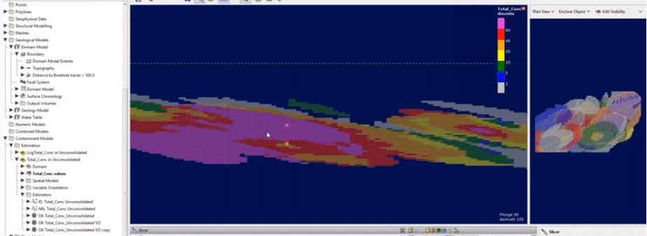
[00:08:02.340]In this project today,

[00:08:03.390]we have a series of geological models.

[00:08:07.020]On the screen, we are looking at a geology model,

[00:08:10.210]which is modeled lithology, so we’ve got bedrock

[00:08:13.870]and some unconsolidated sediments split

[00:08:16.940]into three different units,

[00:08:19.260]and we have a set of boreholes

[00:08:21.390]with a total concentration of contaminant element.

[00:08:26.500]Now within this data set, there’s no continuous sampling,

[00:08:30.680]so it tends to be just one sample per borehole

[00:08:35.400]that has been measured.

[00:08:38.950]So the first thing we need to do is,

[00:08:41.083]then also as well as that, we also have a water table model.

[00:08:46.350]And in this instance, we’ve got the bed

[00:08:49.270]above the water table has been divided

[00:08:51.650]into a vadose side and a saturated side.

[00:08:55.350]And see that there are samples scattered

[00:08:58.160]within both of those domains.

[00:09:00.530]There’s very little sampling down in the bedrock

[00:09:03.430]or below the water table.

[00:09:06.403]To get an appreciation on whether there’s any relationship

[00:09:10.680]between particular units and the underlying contaminants,

[00:09:14.600]we can use some statistical tools.

[00:09:18.210]So we’re up in our borehole data,

[00:09:21.970]and we can use the merge table facility to join

[00:09:28.455]our assay data with the underlying models.

[00:09:31.870]So in this case, I’ve got the geology model

[00:09:34.310]to end up with the contaminant and then the water table.

[00:09:38.380]So if I want to have a look at the statistics,

[00:09:40.950]I right click and there’s Statistics,

[00:09:43.610]and this gives us a variety of options.

[00:09:45.400]We can look at the table statistics,

[00:09:47.640]we could look scatter plots,

[00:09:49.056]and box plots are particularly useful

[00:09:51.780]for this kind of thing.

[00:09:53.180]So looking at a box plot of the geology

[00:09:55.800]and the contaminant of interest,

[00:09:57.610]which is in this case called total concentration,

[00:10:00.460]we can see that the outwash and ice deposits and the till

[00:10:05.390]has the greatest concentration of the contaminant

[00:10:08.410]and bedrock and the outwash deposits, not so much.

[00:10:13.410]If we want to have a look at it relative to the water table

[00:10:17.990]and have a look at another box plot,

[00:10:20.010]and we can see here that there seems

[00:10:22.570]to be a greater concentration in the saturated zone

[00:10:25.580]versus the vadose side,

[00:10:27.300]and there isn’t very much happening down in the bedrock.

[00:10:30.780]These tables can be easily manipulated.

[00:10:34.480]You can turn things on and off,

[00:10:36.200]and the graphs are easily copied

[00:10:39.790]from a copy of the image

[00:10:41.570]so that you can place them directly into a table.

[00:10:48.360]If we want to look at all of that together

[00:10:49.970]and see what the actual values are,

[00:10:52.070]then we can look at table of statistics.

[00:10:57.070]So in this case, I’m looking at the geology model,

[00:11:00.820]so I’ve added that in and the water table.

[00:11:04.270]And within that, I’ve selected the units of interest.

[00:11:06.740]So if I did want to look at outwash deposits as well,

[00:11:09.150]I can click that on.

[00:11:11.130]So I’m looking at domain

[00:11:13.630]of all my concentrate of my contaminant.

[00:11:17.600]We can see that the bedrock’s got very little

[00:11:20.560]and generally the saturated zone

[00:11:23.770]has a greater concentration than in the vadose side

[00:11:27.800]for both the till and the outwash.

[00:11:31.870]There’s very little samples in the outwash deposit,

[00:11:35.330]it’s only three, so it’s unlikely

[00:11:37.610]that we would want to try and estimate that by itself.

[00:11:40.003]There’s not enough data.

[00:11:42.750]So for the purpose of this exercise,

[00:11:45.980]we’ve decided to domain out

[00:11:48.760]the unconsolidated sediments from the bedrock

[00:11:51.410]and not split it out between the vadose and saturated zone,

[00:11:55.230]but that’s always something

[00:11:56.110]that could be done later as well if necessary.

[00:12:01.717]Again, any of these tables can be selected

[00:12:05.820]and copied and pasted into a report,

[00:12:08.390]or we can export them as a CSV.

[00:12:13.540]So for the purposes of this model,

[00:12:18.560]we’re actually just looking at two domains,

[00:12:21.010]and we’re only going to estimate

[00:12:22.970]inside the unconsolidated sediments,

[00:12:25.970]which is the yellow unit on the screen.

[00:12:29.240]The estimation processes is all constrained

[00:12:31.790]within this Contaminant Models folder.

[00:12:34.050]And you’ll see that there are two subfolders,

[00:12:36.230]an Estimation folder and a Block folder,

[00:12:38.990]sorry, Block Models folder.

[00:12:42.080]All of the parameters are set up

[00:12:44.340]and is done in the Estimation folder,

[00:12:47.270]and then we run and view the results

[00:12:49.230]from using a block model.

[00:12:52.040]So we can create a new contaminant estimation.

[00:12:55.610]If we already have one there, we can just open it up.

[00:13:02.070]So the key for this

[00:13:03.570]is that we do need a domain of some kind,

[00:13:07.380]so we either have a volume

[00:13:10.240]that’s been inside a Leapfrog Works geological model

[00:13:13.650]or we can have meshes directly.

[00:13:16.270]So if we have imported a mesh from elsewhere,

[00:13:19.470]you can use that as the domain.

[00:13:22.530]And you can see here that any valid meshes,

[00:13:26.320]they’ll be closed, our value to choose from.

[00:13:29.570]So we’re using this, unconsolidated sediments,

[00:13:32.950]and then we’re using the total concentration values

[00:13:36.440]from the original drillhole table.

[00:13:39.520]Again, you can choose any numeric column

[00:13:42.530]from any of your drillhole database,

[00:13:45.620]and if you have a point data in the Points folder,

[00:13:48.730]that would be available here as well.

[00:13:51.810]Once we’ve chosen the field of interest,

[00:13:54.570]we do have compositing options.

[00:13:56.780]Because this data is only one and they’re all per hole,

[00:13:59.470]we do not need to do that,

[00:14:01.130]but we have all the standard compositing tools

[00:14:04.190]that are really used in the industry.

[00:14:07.070]So we can do it either by whole drillholes

[00:14:09.770]or within the boundaries that you’re working with.

[00:14:13.800]This gives us straightaway an idea

[00:14:15.700]of the distribution of your data,

[00:14:18.560]and then it will also conduct a boundary analysis,

[00:14:21.520]which is looking at our domain inside and outside.

[00:14:25.760]This is used to determine, do we want to use

[00:14:28.970]any of the samples outside of the domain boundary

[00:14:31.700]to help influence the estimate around the edges?

[00:14:35.360]Most of the time you don’t, but sometimes with marginal,

[00:14:40.320]we may have fuzzy boundaries on your domains,

[00:14:43.480]and you may want to look at a few meters outside

[00:14:46.280]to just help inform the estimate there.

[00:14:50.170]In that case, you’d pick a soft boundary

[00:14:52.510]and you can manually decide where you want to go

[00:14:55.320]or just type in meters in the top up here.

[00:15:01.050]At any time, you can go back to your folder

[00:15:05.604]and open it.

[00:15:06.627]And if you want to swap out into a different volume,

[00:15:10.150]you can just pick it,

[00:15:11.120]and everything connected to it will run.

[00:15:15.798]When going within each Estimation folder,

[00:15:17.833]then we have a series of subfolders.

[00:15:22.568]So the first is the Domain.

[00:15:24.020]So we can double check

[00:15:25.650]that that is the domain of interest.

[00:15:29.800]So in this case, it was the unconsolidated sediments,

[00:15:32.560]and this has actually been set up with a distance buffer

[00:15:35.690]of 500 meters from the data points

[00:15:37.900]so that it doesn’t estimate out

[00:15:39.550]into areas a long way from any known data,

[00:15:43.210]and that’s done by the boundary field

[00:15:46.650]within the actual geological model,

[00:15:48.660]so this distance buffer set up here.

[00:15:52.300]We can see our values,

[00:15:54.260]and these are the ones that adjust inside the domain.

[00:15:57.451]So let’s make that transparent.

[00:15:59.723]So what it does, if you’ve got drillhole data,

[00:16:02.660]that then turns it into point data,

[00:16:04.990]so this will be effectively the midpoint of each interval.

[00:16:08.690]And you can display it as normal,

[00:16:11.750]you can put labels on them so you can see the values

[00:16:15.260]to get a feel for how things are running,

[00:16:19.470]and you can do statistics at this level as well.

[00:16:22.200]So before we were looking

[00:16:24.740]at the whole table

[00:16:28.530]and would use flagging from the models to help isolate it,

[00:16:32.990]but once we’re down in the estimation domain,

[00:16:35.810]if we do statistics here, it’s just on that domain.

[00:16:39.560]So these are the samples only within that domain,

[00:16:41.820]so there’s 66 of those.

[00:16:44.057]And all of our graphs are interactive in Leapfrog Works.

[00:16:49.170]So if I bring that here.

[00:16:51.320]If I’m interested in one of these high values above 100,

[00:16:55.040]where are they?

[00:16:56.020]I just highlight the histogram,

[00:16:57.960]and it will show me where those values are.

[00:17:00.660]So I can see that they’re not all clustered in one spot.

[00:17:04.320]If they were, maybe we’d want to subdomain those out,

[00:17:07.580]but they’re not, so we’re leaving this be.

[00:17:11.020]If we wanted to see where the low grade,

[00:17:15.010]these low grade ones are,

[00:17:17.277]it can pop those in and see that, oops,

[00:17:22.160]that only represents two samples in our data set.

[00:17:27.150]So I’ll close that.

[00:17:28.820]If we wanted to look at a low probability plot,

[00:17:31.930]we can just stick it on and it’ll show it in that bit.

[00:17:35.210]Again, we can copy out these images,

[00:17:38.010]and we can also actually copy the data,

[00:17:41.290]so that will copy out this information here,

[00:17:44.850]put it into an Excel spreadsheet.

[00:17:48.950]Okay, so the next component is the spatial models,

[00:17:53.790]and this is where we do the variography.

[00:17:57.680]We create.

[00:17:58.920]We can have numerous models within the same folder.

[00:18:02.550]We might need to compare different variograms

[00:18:07.060]against each other to see how they affect the data

[00:18:10.690]and the estimate,

[00:18:11.840]and once we’ve got a new one,

[00:18:15.240]we then can just open it up to edit it.

[00:18:21.610]Okay, so variography is the analysis

[00:18:25.230]of the spatial variability of the concentration

[00:18:27.790]within the domain.

[00:18:29.770]Some locations may have

[00:18:31.420]very high spatial variability of twin samples

[00:18:34.400]while others may have low variability.

[00:18:36.900]We use the variogram to quantify

[00:18:38.890]the spatial variability between samples.

[00:18:42.260]There are two components to the variogram:

[00:18:45.000]an experimental variogram, and that which is

[00:18:52.130]these represented by the dots,

[00:18:54.920]and then we fit a model to that, which is the fitted curve,

[00:18:59.260]and it’s the curve that we tend to move around

[00:19:04.020]to try and develop these criteria.

[00:19:07.620]So we’re looking for ranges in the different directions,

[00:19:11.040]so this is the major axis, semi major, and minor.

[00:19:14.920]And then the vertical axis represents the sills,

[00:19:18.810]and we tend to have that equal to one.

[00:19:21.370]It’s been normalized to the variance of the data set.

[00:19:25.230]So what we’re mainly interested in is, where are the dots?

[00:19:29.460]Or if they arise from no variability.

[00:19:32.240]This is like at zero distance

[00:19:34.470]if you took a sample right at the same spot twice.

[00:19:39.290]If there’s a little bit of inherent sample error,

[00:19:41.630]we have what’s called a nugget effect.

[00:19:43.780]But the contaminants, it’s generally fairly low,

[00:19:47.060]that we’ve got a low nugget, which is set up in here.

[00:19:51.570]And then as we get further away, so this is 500 meters.

[00:19:54.600]This is 1,000 meters.

[00:19:56.230]This is saying that in the dominant direction,

[00:19:59.890]which we’ll look at in a moment,

[00:20:01.496]by the time we get to around 1,600 meters,

[00:20:04.980]there’s no correlation between any of the samples,

[00:20:07.670]so we don’t really need to be looking beyond that.

[00:20:10.820]The key with Leapfrog is that the graphs are interactive.

[00:20:15.380]Again with the Scene,

[00:20:16.810]and we can always see what our ellipsoid looks like.

[00:20:21.550]So I’ll just turn off our domain, turn off the labels.

[00:20:26.780]So whilst we’re working in the variogram,

[00:20:29.490]we can always see what our orientation ellipsoid looks like,

[00:20:35.050]and it’s interactive.

[00:20:36.610]So here.

[00:20:40.250]So, oops.

[00:20:45.020]So if I click on the ellipsoid itself…

[00:20:48.050]Turn off these structures.

[00:20:51.120]I click on it here,

[00:20:52.400]I can see it’s color coded without the axes,

[00:20:54.840]so I’ve got red, green, and blue.

[00:20:56.970]And this is the red axis,

[00:20:59.560]so if I move it in here, it’s going to move in the graph.

[00:21:05.170]Same with the green one. Bring it back.

[00:21:10.040]If I move the little handles

[00:21:13.450]in the graph,

[00:21:15.370]you can see how that’s changing the ellipsoid.

[00:21:18.536]So you can always see

[00:21:21.700]what your result is likely to look like

[00:21:24.000]and whether it still makes sense geologically.

[00:21:26.960]So how do we get an idea

[00:21:29.750]of what may be right?

[00:21:31.360]Well, we usually start off with a point

[00:21:33.790]of just looking at our data.

[00:21:37.190]And, in this instance, it’s a fairly planar data set,

[00:21:40.800]but we might determine that there’s continuity

[00:21:46.180]in this sort of plane.

[00:21:48.770]And maybe there’s a plunge of our concentrates coming down

[00:21:52.500]in that direction, sort of running down through here.

[00:21:55.000]Doesn’t mean it’s exactly right,

[00:21:56.500]but it gives us a starting point.

[00:21:59.070]Then when we’ve opened up our variogram,

[00:22:02.910]we can actually set that from this plane,

[00:22:05.330]and that will set the initial starting point

[00:22:07.880]and we can see whether there is any continuity.

[00:22:10.700]If we get rising points coming up, that’s a good sign.

[00:22:15.970]We do have some data requires a long transform,

[00:22:20.070]which I did on this one, and it gives a better model,

[00:22:25.120]which you can then use in the untransformed data.

[00:22:28.480]So there’s a bit of structure to the variogram here

[00:22:31.370]so that we can get our model,

[00:22:32.900]and then we can help use these parameters

[00:22:36.310]to guide development of other variograms.

[00:22:39.360]Once it’s all been set up, we hit the Save button,

[00:22:42.650]and then those variograms are available

[00:22:44.530]to be used inside an estimation.

[00:22:48.710]So the Estimator is the most important folder.

[00:22:52.230]There’s Estimators here.

[00:22:54.660]And we can set up four different types.

[00:22:57.450]We’ve got inverse distance, nearest neighbor, kriging,

[00:23:01.943]and we have ordinary kriging and simple kriging.

[00:23:05.680]And we can still use the RBF here too to collect,

[00:23:10.560]which is the same one that’s been used

[00:23:12.100]in the numeric modeling functions

[00:23:14.070]of Leapfrog Works for quite a long time.

[00:23:17.180]So we’re going to have a look at the ordinary kriging set up.

[00:23:21.250]Set up for each of these estimators

[00:23:22.840]is very similar for everyone.

[00:23:25.450]So it picks the variogram,

[00:23:27.846]and it can see any variogram model

[00:23:29.543]that we have within the same folder.

[00:23:31.950]And this, I guess I just have the one.

[00:23:36.650]So the ellipsoid is we set it

[00:23:40.010]to the correct variogram.

[00:23:42.540]So now we’ve picked it in front of here.

[00:23:45.040]It doesn’t necessarily align it straightaway,

[00:23:47.920]so you should always go in and just make sure

[00:23:50.950]that you’re picking the right variogram model.

[00:23:53.890]That will pick up the ranges and the orientation,

[00:23:58.140]and then we know we’re good to go.

[00:24:01.210]The search field, we just say how many samples

[00:24:04.400]minimum we need to estimate a block and maximum.

[00:24:08.000]And again, in real world, you could copy this one

[00:24:11.500]and try different parameters here, like four,

[00:24:14.230]if data, et cetera.

[00:24:15.300]Sometimes it makes it quite a difference

[00:24:17.960]to how many samples you select to a outcome.

[00:24:22.270]And in the Outputs, we automatically can store

[00:24:25.240]any of these variables if we tick the box.

[00:24:28.820]So if we want to use kriging variance,

[00:24:31.420]kriging efficiency, or slope of regression as a guide

[00:24:34.410]for how good the estimate may be, we just tick these on,

[00:24:38.250]and it will store those variables in our block model for us.

[00:24:41.980]I’m going to be using average distance

[00:24:43.880]as an aid for classification

[00:24:46.030]in terms of indicated, measured, and inferred,

[00:24:49.030]so I’m going to tick that on because I want to use it.

[00:24:52.240]Generally if I don’t want to use the output,

[00:24:54.710]I don’t tick it on.

[00:24:56.010]It just keeps things tidy down the track.

[00:25:00.010]And then the actual name of the variable will be

[00:25:02.150]whatever we type in here.

[00:25:03.840]That puts in a default,

[00:25:04.870]but you can change that to something simpler.

[00:25:10.010]We can copy these, so I can go to Copy,

[00:25:13.240]and then you can change some of the parameters slightly,

[00:25:16.350]and then you’d be able to compare the results

[00:25:18.290]on different estimators.

[00:25:21.880]We also have what’s known

[00:25:23.980]as a variable orientation function.

[00:25:31.440]Within this, what I’ve done here is

[00:25:37.670]put in a mesh that’s showing us the potential

[00:25:42.460]for a slight kink and warping within the layer,

[00:25:45.800]so it doesn’t have to be planar.

[00:25:48.350]So without variable orientation,

[00:25:51.840]you were basically using the ellipsoid that you’ve defined,

[00:25:56.570]and so every place and when it estimates,

[00:25:59.840]every block is using this orientation.

[00:26:02.710]But we can see here that we’ve got

[00:26:04.820]sort of variability across that way.

[00:26:10.940]We can see that there is flatter design within here

[00:26:14.817]and a little bit steeper in through there.

[00:26:16.990]So then that means that if we had

[00:26:18.560]a more horizontal ellipse in this area,

[00:26:20.720]it might select samples better

[00:26:23.490]to give a slightly better estimate.

[00:26:25.680]We can visualize that orientation.

[00:26:27.950]So this is looking at the variable orientation

[00:26:32.780]as functional dip,

[00:26:34.920]so we can say that we’ve got a flatter dipping zone

[00:26:37.810]right through the middle here.

[00:26:39.660]We can use any open mesh

[00:26:43.720]to help define this variable orientation.

[00:26:47.240]In this Variable Orientation folder,

[00:26:49.600]we just select the mesh of interest, and then I’ll just,

[00:26:53.080]this is the visualization of it using the discs.

[00:26:58.010]If we want to apply that variable orientation,

[00:27:00.850]I’ve copied this kriging estimator

[00:27:05.670]and in the ellipsoid,

[00:27:08.730]originally that was the variogram,

[00:27:11.280]and then I just take this variable orientation

[00:27:13.660]and pick the one that I’m interested in.

[00:27:15.770]Again, you can set up a number

[00:27:19.100]of different variable orientations

[00:27:20.500]to test against each other,

[00:27:21.740]and you would just build up multiple estimators

[00:27:24.190]using each one.

[00:27:27.590]So we’ve now set up a series of estimators,

[00:27:30.050]and we’re ready to try and apply these,

[00:27:34.300]make an estimate.

[00:27:36.030]And this is all done in the Block Models folder.

[00:27:40.230]So to make a new block model,

[00:27:41.780]we would just go to New Block Model

[00:27:43.403]and define the parameters.

[00:27:45.600]Once it’s been defined, we can open it.

[00:27:48.190]And, again, you can do this at any time

[00:27:50.570]and come back and change things.

[00:27:52.690]It’s very similar to setting up the geological model.

[00:27:57.880]You would share your data generally.

[00:28:04.900]I’ll just bring that in.

[00:28:07.660]So there’s the data points there,

[00:28:10.400]and just make sure that we’re covering,

[00:28:12.140]but I generally enclose my object to make sure

[00:28:14.970]that it matches exactly my geology modeling stents,

[00:28:18.110]and then everything is aligned.

[00:28:20.330]We can rotate

[00:28:23.870]a block model in Azimuth.

[00:28:25.390]So if we had a 45 degree

[00:28:27.920]trending deposit of interest,

[00:28:30.740]well, then we can rotate that to 45 degrees,

[00:28:36.650]and set it up accordingly.

[00:28:40.210]So I’ll that back to zero.

[00:28:42.270]Okay, the the key concept

[00:28:45.080]of Leapfrog Works is evaluating to the block model.

[00:28:49.970]So everything that’s stored

[00:28:53.530]in the Estimation folder will initially sit over here

[00:28:56.580]on the left-hand side.

[00:28:57.690]It’s similar to when we’re working with merge tables.

[00:29:00.610]all our tables would be over here,

[00:29:02.880]and the things that we want to join together

[00:29:05.030]that we’ll look at are shifted out to the right-hand side.

[00:29:08.530]So I want to look at all of my core estimators together

[00:29:11.727]’cause I want to compare the results from all four,

[00:29:15.060]but if I’m not interested in nearest neighbor,

[00:29:16.940]which is mainly used as a validation tool

[00:29:19.050]not as an actual reporting value, I can take that out.

[00:29:24.040]Again, you can add and remove things at any time,

[00:29:26.880]and it’ll just rerun.

[00:29:29.830]If we want to report on, say, geology

[00:29:32.630]or whether it’s in the saturated or vadose side,

[00:29:36.160]we do need to bring across the domains

[00:29:38.330]from our geological models.

[00:29:40.210]So generally you will bring across the whole geological,

[00:29:43.690]we can only bring across the whole geology model,

[00:29:46.260]and that’ll give you the option later

[00:29:47.960]of selecting individual volumes from that to report against.

[00:29:54.120]So if you create a new estimator in here,

[00:29:58.140]so if I came back here and I just copied this one,

[00:30:06.290]so now I’ve got a copy.

[00:30:07.440]If I cancel this and open it again,

[00:30:12.720]you’ll see that it’s sitting over on the left-hand side.

[00:30:17.300]And then if I want to run it,

[00:30:18.377]I will just bring it across to that side there.

[00:30:22.210]Okay, so that’s how we create the block model.

[00:30:26.440]And by going OK, that is running the estimate.

[00:30:29.060]There’s no separate run buttons or anything like that.

[00:30:31.700]Basically it’s run and ready to go.

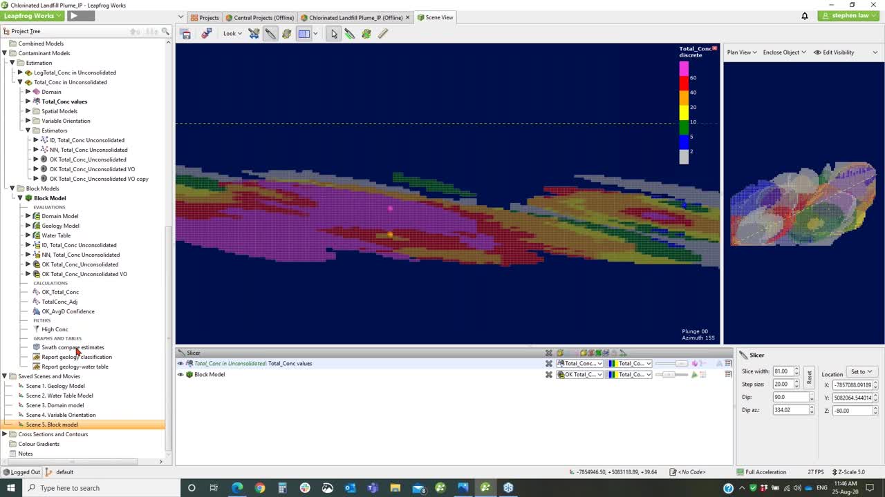
[00:30:34.160]So to look at it, we drag it into the Scene,

[00:30:37.850]and we can see the results,

[00:30:40.550]which looks a little bit odd in that orientation.

[00:30:43.520]Now to view, basically we can see any

[00:30:47.010]of the variables that we chose.

[00:30:48.710]I want to look at inverse distance.

[00:30:50.670]I just tick on it, and it’ll show it to me.

[00:30:53.283]I want to look at the kriging result.

[00:30:58.010]That’s it there.

[00:31:00.210]We also have this Status button, which can be useful.

[00:31:03.040]It shows us which blocks are actually estimated.

[00:31:06.644]If I edit and turn off without value on,

[00:31:09.760]we can see that the purple blocks

[00:31:11.540]don’t actually have a value estimated into them

[00:31:14.070]and white ones do, and that can be helpful for determining

[00:31:18.830]whether we need to do anything slightly different.

[00:31:21.050]I didn’t want these other blocks estimated at this stage,

[00:31:25.770]so I’m just turning that off so I can’t see them.

[00:31:31.513]Another application for block models

[00:31:35.140]is calculations and filters.

[00:31:37.490]I right click on here, I go Calculations and Filters,

[00:31:41.010]and we this whole system of being able

[00:31:44.250]to build quite complex calculations based on any

[00:31:48.450]of the variables stored within the block model.

[00:31:51.720]So this shows us

[00:31:55.590]everything available to us.

[00:31:58.683]Let’s bring that out here for a sec.

[00:32:00.460]So this is showing us what’s stored in the model.

[00:32:03.690]So we’ve evaluated our geology models,

[00:32:06.037]and it means that we can actually use components.

[00:32:08.960]So up here, I would find the porosity variable,

[00:32:11.840]decide that if the domain model equals till, it’s 0.25.

[00:32:17.460]And to create the new ones, it’s quite simple.

[00:32:22.490]Let’s go to there.

[00:32:24.700]And we can put in an if statement.

[00:32:26.550]So we’ve got a heap of syntax helpers over here

[00:32:28.950]on the right-hand side.

[00:32:31.280]And then I just simply select

[00:32:33.480]the domain model equals, say, bedrock,

[00:32:37.700]and then I can put in a value.

[00:32:39.260]So it’s quite easy to build up these calculations.

[00:32:43.450]Once they’re all built,

[00:32:44.780]they can be transferred between block models.

[00:32:49.890]Generally in the same area, you might have multiple models,

[00:32:53.160]but then we would try and keep the same structure.

[00:32:56.190]So we could export

[00:32:59.990]all the items into a file here,

[00:33:02.210]and it goes to a little CAB file.

[00:33:07.420]And then when we go into a new block model,

[00:33:09.870]we can just import that file,

[00:33:12.260]and it saves us having to rebuild all this from scratch.

[00:33:15.920]If there are any variables missing,

[00:33:17.610]say the next model doesn’t have unconsolidated sediments,

[00:33:21.490]it’ll just put a red squiggly line under there

[00:33:23.640]and highlight that that’s missing,

[00:33:25.260]and you can replace it with the correct version.

[00:33:28.310]It’s useful for assigning things

[00:33:32.150]like, in this case,

[00:33:33.670]I’m using average distance that we’ve stored in the model.

[00:33:37.040]If it’s less than 500 meters, it’s measured.

[00:33:39.830]It’s got less than 1,000, it’s indicated, and et cetera.

[00:33:43.370]And any calculation that we’ve made

[00:33:46.060]is immediately visible

[00:33:49.560]in the block model, so you’ll see that here, calculations,

[00:33:52.760]and I can look at my confidence level there,

[00:33:55.327]and we can see it displayed straightaway.

[00:34:03.110]So the last step is validating our results.

[00:34:06.910]So the key one always

[00:34:09.050]is looking at the data,

[00:34:12.400]so looking at the blocks against that data visually,

[00:34:15.610]and the colors of the samples

[00:34:19.250]should be similar or close to the underlined blocks.

[00:34:23.620]So as we move through there,

[00:34:25.290]we can see that there’s not a lot of data in this one,

[00:34:29.060]but we can see here that where we’ve got highs.

[00:34:33.360]We’re getting highs with lows.

[00:34:35.750]It’s also showing me my orientation,

[00:34:38.400]and that’s making sense relative to what I expect.

[00:34:42.202]If it was striped in the opposite direction,

[00:34:45.340]then it would suggest I’ve made an error in my orientation,

[00:34:49.130]in the variogram, and I can go back and check.

[00:34:52.500]One of the things we can do

[00:34:54.410]is interrogate down to the block level.

[00:34:56.900]So if I click on any block

[00:34:59.840]and use this Interrogate Estimator, it will show me

[00:35:04.790]for the variable orientation estimator

[00:35:09.600]that I have found this many samples,

[00:35:13.440]and we’ve got to include,

[00:35:15.060]so I said I would use up to 10 samples,

[00:35:17.693]so it’s only found 7.

[00:35:20.330]It meets the minimum criteria of needing two at least.

[00:35:23.730]That’s used all of these samples. These are the grades.

[00:35:26.800]These are the distances from the data point,

[00:35:29.317]and you can sort by that.

[00:35:32.070]And it’s saying that the average value ended up being 93.

[00:35:35.750]We can view that in the screen.

[00:35:39.540]So I’ll just turn off the ellipse for a second.

[00:35:42.040]So we’re looking at our block,

[00:35:44.380]and it’s showing me there’s the samples

[00:35:46.040]that are being used to inform that block.

[00:35:50.800]If there’s something wrong,

[00:35:51.990]say we’ve got a really high sample

[00:35:53.950]that we don’t want to inform that block,

[00:35:55.880]we could go directly back to the estimator

[00:35:59.740]and change up a couple of parameters

[00:36:02.570]and maybe change the search down a little bit.

[00:36:05.050]If it’s looking too far,

[00:36:07.060]we might want it to look 1,000 meters,

[00:36:09.270]and see if we can change it in that way.

[00:36:13.030]It will rerun it instantly,

[00:36:14.620]and you’ll be able to see the results interactively.

[00:36:19.400]Also, I’ll filter the block model.

[00:36:24.200]This shows how the variable orientation is working.

[00:36:28.570]Let’s go back here.

[00:36:32.010]So if I click on here, it shows me my ellipsoid,

[00:36:37.080]and if I click over here,

[00:36:39.060]you can see that the ellipsoid is moving around

[00:36:43.560]in the local direction, depending on what.

[00:36:46.240]So it’s a bit flatter in this area over here

[00:36:49.370]than it is up through there,

[00:36:52.060]whereas if we weren’t using variable orientation,

[00:36:54.540]then we would just have this ellipsoid or points.

[00:36:56.740]So you get a good idea on how it’s finding its data.

[00:37:02.240]Okay, we can also look at statistics

[00:37:04.350]or the actual block model.

[00:37:06.030]So again, we right click on the block model

[00:37:07.757]and go to Statistics.

[00:37:09.950]If we look at a table of statistics, it’s down here.

[00:37:15.950]Again, you’ve got lots of choice.

[00:37:18.340]You just add in the models

[00:37:23.200]that you want,

[00:37:24.033]so you could add in extras if you’ve got more.

[00:37:26.690]There’s that one.

[00:37:28.670]Once within the model, I can determine,

[00:37:30.590]I don’t want to look at bedrock or I do,

[00:37:32.600]so that will bring bedrock back in for me.

[00:37:35.030]We didn’t estimate bedrock, so there’s no data there,

[00:37:37.770]so it’s no point being on it.

[00:37:40.210]So it’s broken up by lithology

[00:37:44.930]and then the water table so we can get an idea.

[00:37:49.040]Then we can see that in the saturated side,

[00:37:52.080]the values are quite high,

[00:37:54.220]and in the vadose side, it’s about half that.

[00:37:57.960]And if we went back to our original statistics,

[00:38:00.440]we’d find that they’re similar values.

[00:38:02.400]And that’s one of the main checks.

[00:38:04.170]Other values we’re getting from our raw data in the domain

[00:38:07.740]in the range of what we’re estimating, as they should be.

[00:38:12.420]You can turn on and off things that you don’t want to see.

[00:38:16.880]So another one is swath plot.

[00:38:21.760]So everything is stored in the block model.

[00:38:24.510]So as soon as you update any new data,

[00:38:27.520]so if I add a new borehole in,

[00:38:29.750]and it will update the geological model

[00:38:31.850]as it does in Leapfrog Works.

[00:38:34.000]In the same dynamic workflow works for the block model,

[00:38:37.070]it’s already linked through,

[00:38:38.400]and it will update the block model straightaway.

[00:38:42.540]If we can look at a swath plot, once you’ve made a new one,

[00:38:46.010]it’s visible and retained in the block model down here.

[00:38:49.910]So I can open that up.

[00:38:51.950]You can have as many of these as you like.

[00:38:54.200]So what we’re doing here is swath plot is simply looking at

[00:39:00.270]what’s called swaths.

[00:39:02.050]So I’m looking in the,

[00:39:04.114]if I look in the Z direction and I’m looking north,

[00:39:06.520]I can see here these slices.

[00:39:08.930]And these align with the block model slice,

[00:39:11.250]so there’s a five meter blocks in the Z.

[00:39:13.770]And it’s basically summarizing all the data points

[00:39:16.680]within that slice and giving an average,

[00:39:19.770]and it’s comparing them against the underlying sample data,

[00:39:23.310]which is the red line here.

[00:39:25.000]And what we find is the sample data can be quite erratic,

[00:39:28.710]but the estimates will smooth it out,

[00:39:30.520]and they usually Y set when the data’s like this.

[00:39:35.030]So we can see that all the different estimates,

[00:39:37.650]the inverse distance and the two different krigings,

[00:39:40.350]are fairly similar.

[00:39:41.240]There’s some local variation.

[00:39:43.570]And then the gray one is nearest neighbor,

[00:39:45.580]which is like a check.

[00:39:47.860]Generally estimates shouldn’t be too far away,

[00:39:50.430]especially they shouldn’t go too much

[00:39:52.020]above the nearest neighbor.

[00:39:54.570]We can turn on volumes.

[00:39:56.310]So the reason why this looks a bit odd

[00:39:57.900]is that there’s very little volume here,

[00:39:59.880]so you can get some outlier

[00:40:04.050]sort of things happening around the edges.

[00:40:06.860]And we’re looking in the X direction.

[00:40:09.810]I’ll just turn off those again.

[00:40:11.330]So it can look in the X direction,

[00:40:13.330]the Y direction, and the Z direction.

[00:40:16.670]And they’re all looking fairly okay,

[00:40:18.270]so that’s another good check

[00:40:20.000]for the quality of the estimate.

[00:40:23.410]And the last thing we want to look at is reporting.

[00:40:26.420]So again, we might report in the block model.

[00:40:29.480]So we’ve got New Report,

[00:40:31.720]and you can have as many reports as you like.

[00:40:34.490]So the first one I’m looking at

[00:40:37.260]is just looking at the geology model

[00:40:40.110]broken down by water table.

[00:40:42.020]And then the lithology, it’s giving us the totals,

[00:40:45.350]and this is a cut off of two.

[00:40:47.720]With density, we can have constant values,

[00:40:50.420]but if we estimated it into the model, then we could select.

[00:40:54.150]It would show up in here and we could select that.

[00:40:58.040]Or you can make a calculation of SG,

[00:41:00.740]assigning a different density to per unit,

[00:41:04.840]and then you could use that one.

[00:41:07.410]If you wanted to look at the geology first

[00:41:09.890]and then the water table, you just move the columns around

[00:41:13.240]so it’s looking the way you want it to.

[00:41:15.700]There’s no Save button.

[00:41:16.780]It just automatically saves these reports,

[00:41:19.000]and you just give it a name up here.

[00:41:21.200]And then if we look at the second one,

[00:41:23.740]I’ve added classification in.

[00:41:25.490]So basically that’s where we’ve needed

[00:41:27.650]to bring in the geology models for the domains,

[00:41:31.260]but the calculation shows up here as a category,

[00:41:35.640]which can be used in here as confidence.

[00:41:38.600]And if we want that to be primary,

[00:41:40.620]we can bring it over to the left-hand side

[00:41:43.450]and turn things off.

[00:41:44.283]If we don’t really care about unclassified,

[00:41:47.310]we can just turn it off, if you don’t want to show.

[00:41:50.470]So that’s pretty much the end of the demonstration.

[00:41:55.690]<v Aaron>Fantastic. Thank you very much, Steve.</v>

[00:41:57.850]If you’d like to trial the Contaminant extension

[00:42:01.610]or if you’d like any other information

[00:42:03.790]about the Contamination extension

[00:42:05.580]or any of the other Seequent solutions,

[00:42:08.080]please either go to our website at seequent.com

[00:42:12.210]or contact us at [email protected].

[00:42:16.030]And we have some information on the website

[00:42:18.740]and a link to request trials,

[00:42:20.992]or we’ll help you directly if you email us as well.

[00:42:24.110]So one question we have, Steve,

[00:42:26.810]is are there cross validation tools?

[00:42:31.440]<v Steve>Well, it’s not cross validation tools directly.</v>

[00:42:35.300]The way it’s set up is more

[00:42:37.170]if we wanted to do something like that,

[00:42:40.480]then we would just modify our estimation.

[00:42:43.950]We would set up an estimator

[00:42:46.770]with slightly different criteria.

[00:42:49.540]So we do have the capability within the Estimation folder,

[00:42:53.650]open it up, that you can apply query filters.

[00:42:57.550]So you could exclude some of the data

[00:43:00.810]and run an estimate of that,

[00:43:02.260]and then it’d have one with it included

[00:43:03.940]and get a feel for what impact that is having.

[00:43:07.150]The same as sensitivity analysis.

[00:43:09.140]So the parameters that we were trying to work out,

[00:43:12.210]and actually we’ll use a two, four, six,

[00:43:14.780]or eight minimum number of samples.

[00:43:16.820]We would just set out four different estimates with those,

[00:43:19.950]and then we would plot the results onto this one,

[00:43:22.457]but we’ll get a good idea of what the sensitivity

[00:43:26.250]of having that different parameter would be.

[00:43:29.970]<v Aaron>And correct me if I’m wrong, Steve,</v>

[00:43:30.803]because it’s so quick to do multiple iterations like that,

[00:43:34.250]it can be done very quickly ,

[00:43:35.940]and you can go through that check process.

[00:43:38.730]Is that right?

[00:43:40.150]<v Steve>Yup, it’s quite simple.</v>

[00:43:41.470]And also because once you built out one estimator,

[00:43:45.810]’cause you can just copy them,

[00:43:47.400]so you can just right click, Copy,

[00:43:50.610]it will copy those parameters,

[00:43:52.800]but also you can copy the whole folder.

[00:43:54.820]So you can copy the whole thing,

[00:43:57.860]and you might just change one parameter or even a domain,

[00:44:01.710]and then every estimator that you’ve set up for that,

[00:44:04.630]so we’ve set up five, four here,

[00:44:07.483]they would all be duplicated for the other domain

[00:44:10.127]but set for the other data.

[00:44:12.690]Then you would just need to check the variogram probably,

[00:44:15.310]and once that’s sorted, everything else flows through.

[00:44:18.440]So once it’s all set up,

[00:44:20.050]yeah, the actual process of re-putting in new data

[00:44:24.340]and will be tweaking is quite quick and simple.

[00:44:28.840]<v Aaron>Awesome. Thank you, Steve.</v>

[00:44:31.590]Another question we have is,

[00:44:33.600]is it possible to generate content contours

[00:44:36.670]from the block model?

[00:44:38.390]So I guess there’s a couple of answers to this,

[00:44:40.580]and I’ll let Steve dive into it in a second.

[00:44:42.690]You can generate contours

[00:44:44.110]from any of the surfaces in Leapfrog

[00:44:45.690]using the Contours function in the Cross Section folder.

[00:44:48.760]And otherwise you can, you know,

[00:44:50.550]maybe what you’re also asking there is,

[00:44:52.320]is evaluating those onto a cross section to display as well,

[00:44:55.360]which I think Steve has an example there,

[00:44:59.218]but did you have anything else to add to that, Steve,

[00:45:01.322]on contours from the block model?

[00:45:04.450]<v Steve>We can’t generate grade shells</v>

[00:45:06.860]directly from the block model.

[00:45:08.860]The only way we can do it at the moment

[00:45:11.220]is we would run a RBF estimator.

[00:45:14.510]So we’ll set up, oh, yeah, so there’s an RBF estimator,

[00:45:19.050]which is very similar to numeric models,

[00:45:21.360]that will run a series of contours.

[00:45:23.810]And then we can plot the results

[00:45:27.760]from the RBF interpolate onto the block, onto a section.

[00:45:33.110]<v Aaron>Fantastic. Thanks, Steve.</v>

[00:45:35.350]Another question we’ve gotten here is,

[00:45:37.910]with the multiple estimation methods,

[00:45:41.090]is there any preferred method

[00:45:43.000]or is there much difference between them?

[00:45:46.620]<v Steve>It all comes down to the data set</v>

[00:45:48.900]that you’re working with and there is no right or wrong,

[00:45:52.810]but generally in early stages if the data is quite sparse,

[00:45:56.370]it can be difficult or impossible to get a variogram,

[00:45:59.770]so we would tend to run with things

[00:46:01.480]like inverse distance methods at that level.

[00:46:04.510]But as the amount of data builds up,

[00:46:06.617]we should be able to develop a variogram,

[00:46:09.450]and then ordinary kriging is the go-to one

[00:46:12.880]at this stage usually.

[00:46:14.410]It’s been around for 30 years or more

[00:46:16.900]and it’s quite a robust method,

[00:46:18.960]so it, yeah, it really comes down to what data you’ve got,

[00:46:23.520]but any of the methods are valid.

[00:46:25.920]Nearest neighbor isn’t generally used for reporting

[00:46:29.030]’cause it’s just taking the nearest sample,

[00:46:31.210]but it is a good fill of data.

[00:46:34.390]<v Aaron>Fantastic. Thanks, Steve.</v>

[00:46:36.470]We’ll leave it there for the questions.

[00:46:38.970]If you are interested in some further information,

[00:46:41.780]you can always contact us at [email protected].

[00:46:45.370]For any information on the Contamination extension

[00:46:47.890]or any of our other solutions,

[00:46:49.730]you can go to the Seequent website at seequent.com.

[00:46:53.210]We also have a wealth of online information

[00:46:55.440]at my.seequent.com,

[00:46:57.290]where you can look at the training manual

[00:47:00.020]for various products, including the Contamination Kit.

[00:47:03.470]There’s some useful tips and tricks amongst other things.

[00:47:07.170]We also have a series of upcoming webinars and events,

[00:47:10.390]which you can find at seequent.com/events.

[00:47:13.460]Again, thank you all for your time today.

[00:47:16.270]That’s the end of the webinar,

[00:47:17.390]and we look forward to hearing from you soon.