Technical Tuesday: Drillhole Data Tips for Leapfrog

Zoe will present workflows and go over precautions to consider when setting up your drillhole database in Leapfrog before you commence modelling. Drillhole interval data can be imported into Leapfrog via .csv files, the Central dataroom, the ODBC Link, or the aQuire Link. Downhole points and structures associated with drillholes can also be imported. Once the drillhole data is within Leapfrog there are many options available for interpreting this data via new columns or tables.

Overview

Video Transcript

[00:00:04.540]
<v Zoe>Welcome to today’s webinar</v>

[00:00:06.040]
on Drillhole Data Tips in Leapfrog.

[00:00:08.850]
My name is Zoe and I’m a senior project geologist

[00:00:11.730]
with Seequent here in Perth.

[00:00:14.410]
There is a lot of flexibility

[00:00:15.970]
when preparing data for modeling in Leapfrog,

[00:00:18.430]
and there’s no right or wrong way to do this.

[00:00:21.610]
What we will present here are some options

[00:00:24.170]
and precautions to consider

[00:00:25.880]
before starting the modeling process

[00:00:28.360]
to ensure you get the best workflow set up

[00:00:30.830]
from the beginning.

[00:00:39.760]
This technical session will cover

[00:00:42.430]
taking a look at importing drillhole data.

[00:00:45.770]
This includes interval data such as logging and assay data,

[00:00:50.114]
downhole points, and downhole structural measurement.

[00:00:54.530]
We’ll look at validating that data within Leapfrog,

[00:00:57.580]
and I’ll point you towards some good resources we have

[00:00:59.980]
about how to deal with error handling.

[00:01:03.900]
We’ll look at how to create new columns within Leapfrog

[00:01:06.530]
from that important data, and how to set up merge tables.

[00:01:11.330]
And finally, once we’ve completed all of these steps,

[00:01:14.430]
how to choose a base lithology column

[00:01:16.750]
for a geological or domain model,

[00:01:19.270]
and how to apply a query filter to this model,

[00:01:21.850]
if appropriate.

[00:01:24.550]
The first step we’ll look at is importing drillhole data.

[00:01:28.690]
Leapfrog Geo can import drillhole data

[00:01:31.030]
from files stored on your computer or network location,

[00:01:35.210]
from a central projects data room, if you have central,

[00:01:39.130]
from any database that runs an ODBC interface,

[00:01:43.130]
or from an acQuire database.

[00:01:46.050]
For any of these options, once the data source is selected,

[00:01:49.650]
the process of importing drillhole data is very similar.

[00:01:53.860]
To start, right click on the drillhole data folder

[00:01:58.000]
and select import drillholes.

[00:02:04.170]
And we’ll navigate to the folder location in this case.

[00:02:11.830]
Leapfrog is expecting a minimum of a collar table,

[00:02:15.290]
survey table, and at least one interval table.

[00:02:21.010]
The survey assay and lithology tables

[00:02:23.860]
will be automatically selected

[00:02:25.550]
if they’re named something sensible.

[00:02:29.540]
We can add additional tables here at this stage

[00:02:32.490]
or remove tables if you don’t want to import them,

[00:02:35.850]
and we can also add downhole points

[00:02:38.310]
at the stage of the import.

[00:02:42.770]
Downhole structures will need to be imported

[00:02:44.760]
once these drillholes are in the project.

[00:02:48.270]
So we’ll click import and check the auto mapping

[00:02:51.770]
or manually map the columns for each of these tables,

[00:02:55.410]
and click next once you’re happy with each table set up.

[00:03:00.210]
The table that you’re working on will be in bold

[00:03:03.610]
up in the progress bar at the top here.

[00:03:07.140]
We won’t go through each column individually

[00:03:09.510]
in this exercise, but I’ll highlight the import as options

[00:03:13.590]
as we step through.

[00:03:17.310]
So the collar table, we’ll select next

[00:03:20.780]
and same with the survey table,

[00:03:22.350]
these columns have been automatically mapped.

[00:03:26.520]
With the assay table, the hole ID from and to

[00:03:30.460]
have been automatically selected,

[00:03:32.890]
but the gold and arsenic values haven’t been selected yet.

[00:03:38.040]
This is where the import as options

[00:03:40.760]
are important to fully understand.

[00:03:43.170]
So we’ll step through those.

[00:03:46.510]
Where it says not imported at the top here,

[00:03:48.820]
we can drop down and choose how to import this column.

[00:03:55.460]
The lithology and categories are used to import

[00:03:58.770]
any categorical data such as lith codes,

[00:04:01.410]
weathering, and alteration,

[00:04:03.840]
and the functionality is equivalent in Leapfrog.

[00:04:07.790]
Text is used to import summary or description columns,

[00:04:12.530]
and columns imported as text cannot be used for modeling.

[00:04:16.400]
So their use is limited within the project.

[00:04:19.650]
I generally only bring in free text fields

[00:04:22.230]
such as logging comments.

[00:04:26.370]
Numeric is used to import any numeric data

[00:04:29.460]
such as assays, temperature, and drop quality designations.

[00:04:34.640]
Timestamp and date are used to import

[00:04:37.870]
time and date information in custom formats

[00:04:40.790]
that are supported with these.

[00:04:44.090]
The URL option is used to import an associated URL

[00:04:48.890]
and can be used to connect core photos,

[00:04:51.230]
which is stored in a directory to the correct drillholes.

[00:04:57.220]
These column types cannot be changed after import,

[00:05:00.500]
so choose carefully.

[00:05:02.350]
However, in the latest version of Leapfrog,

[00:05:04.800]
imported columns can be deleted and re-imported

[00:05:07.950]
if you do happen to bring them in incorrectly,

[00:05:10.890]
and then they can be renamed also

[00:05:12.790]
if you need to remap to a different column here.

[00:05:16.570]
So let’s go through and map the columns

[00:05:18.610]
for these data tables.

[00:05:21.280]
So the gold and arsenic values will come in as numeric.

[00:05:27.380]
Their lithology will come in as lithology.

[00:05:31.610]
We’re now looking at our points file.

[00:05:34.350]
So we’ve got a hole ID, depth,

[00:05:36.210]
and the structure type that’s been logged downhole,

[00:05:39.670]
and that structure type can come in as a category.

[00:05:45.020]
I’ll click finish, and these will come into the project.

[00:05:52.200]
Once the drillholes have imported,

[00:05:54.700]
they will appear in the project tree

[00:05:56.680]
under drillholes object.

[00:05:59.730]
Now that they’re in the project,

[00:06:02.520]
we can also bring in downhole structural measurements.

[00:06:06.550]
These are imported by right clicking on the drillholes,

[00:06:10.060]
choosing import from file, and plano-structural data.

[00:06:15.560]
I’ll select my structure file here.

[00:06:21.410]
And you can see we’ve got hole ID, depths.

[00:06:25.190]
We’ve got dip and azimuth as well as alpha and beta.

[00:06:28.410]
So you only need either or not both.

[00:06:31.940]
I’ll bring in the alpha and beta measurements

[00:06:34.270]
and Leapfrog will automatically convert to dip

[00:06:37.440]
and dip direction.

[00:06:40.530]
I’ve also got a category column here for structure type.

[00:06:43.530]
So I’ll bring that in associated

[00:06:45.300]
with each of those structures and click finish.

[00:06:50.640]
Now that we have the data in our project,

[00:06:52.900]
we can move on to validating our drillholes.

[00:06:58.720]
There is some things we should consider

[00:07:00.510]
when importing data into Leapfrog.

[00:07:03.570]
This isn’t a comprehensive list,

[00:07:05.560]
but is a good starting point to make sure that

[00:07:07.876]
we’re getting the information that we need for our model.

[00:07:13.110]
Do we have any missing assay values

[00:07:15.460]
and how do we want to handle these?

[00:07:18.000]
We’ll talk a little bit later

[00:07:19.500]
about the implications of replacement rules.

[00:07:22.910]
Are there any values that are outside

[00:07:24.670]
the expected range of data, for example, percentages

[00:07:28.190]
or RQD greater than 100?

[00:07:31.500]
Is the spatial position of data correct?

[00:07:34.340]
Are survey files validated and up to date?

[00:07:37.770]
Are there any duplicate points or overlapping intervals

[00:07:40.790]
within our data set?

[00:07:45.380]
Some other things to check in the database

[00:07:47.660]
that may not be picked up by Leapfrog

[00:07:49.630]
or the software that you’re using are listed here below.

[00:07:54.510]
So these are things like does the database contain

[00:07:58.170]
all of the programs drilled?

[00:08:00.310]
Have all relevant assays been returned?

[00:08:03.110]
Were any QAQC issues raised with the recent drilling?

[00:08:07.920]
If there are any missing data intervals, can they be found?

[00:08:12.820]
Does the database contain all of the surface,

[00:08:15.750]
underground, and face-chip data in the same database?

[00:08:19.710]
Has the collar table were being checked for unsurveyed holes

[00:08:22.740]
or holes that haven’t had their collar surveys validated?

[00:08:26.140]
And is there any unusual deviation

[00:08:28.230]
with the diamond drill holes?

[00:08:29.710]
A visual check can often pick this up.

[00:08:33.360]
For face-chip samples, are they correctly positioned

[00:08:36.650]
within as-builts and development?

[00:08:40.080]
And are there any face-chips at unexpected angles

[00:08:42.540]
to development?

[00:08:46.280]
So the common errors and warnings within Leapfrog

[00:08:49.570]
are shown here.

[00:08:51.570]
Some examples include duplicate hole ID errors.

[00:08:55.600]
The hole ID is missing from the collar table

[00:08:58.080]
that will throw up an error,

[00:08:59.800]
and if column max depths are exceeded in interval tables

[00:09:02.763]
that will also throw up an error.

[00:09:06.100]
If the from depth exceeds the to depth

[00:09:09.070]
or there are any overlapping segments,

[00:09:11.060]
this will show up as an error in Leapfrog,

[00:09:13.880]
and Leapfrog will also identify

[00:09:15.920]
if there are potential wedge holes.

[00:09:21.010]
As well as these common errors and warnings,

[00:09:23.840]
Leapfrog will also pick up invalid values

[00:09:26.550]
in numeric columns.

[00:09:28.230]
And let’s have a quick look at our assay table here.

[00:09:36.720]
So we don’t have any errors in this dataset,

[00:09:39.200]
but we do have a couple of warnings.

[00:09:42.090]
So that’s saying there are no values

[00:09:44.370]
for these certain hole IDs,

[00:09:46.810]
and we do have some invalid value handling issues.

[00:09:49.770]
So we’ll take a look at gold here.

[00:09:53.540]
We’ve got missing intervals and missing values.

[00:09:57.380]
We don’t have any non-numeric values, so that’s fine,

[00:10:00.280]
but these will also be picked up.

[00:10:01.870]
So for example, a less than symbol in your database.

[00:10:07.130]
And we don’t have any negative values

[00:10:09.140]
or non-positive values here in this dataset either,

[00:10:11.677]
but these will be picked up too.

[00:10:15.530]
We can choose how we want to handle

[00:10:18.220]
these missing intervals and values.

[00:10:20.430]
Can either omit them or replace them.

[00:10:24.271]
In this case, I’m going to admit to them

[00:10:27.590]
and say that these rules have been reviewed,

[00:10:30.290]
and same here for the arsenic.

[00:10:33.860]
We’ve got missing intervals and values

[00:10:35.850]
so they can be omitted.

[00:10:38.540]
And the non-positive values, we’ve got a 0.0,

[00:10:43.000]
and I’ll just keep that one in the dataset.

[00:10:48.680]
Saving those rules will remove the red flag

[00:10:52.260]
from this assay table.

[00:10:56.260]
If any errors or inconsistencies are detected in your data,

[00:11:00.350]
aside from these invalid value handling rules,

[00:11:03.610]
then these must be fixed in the original database

[00:11:06.480]
and reloaded into Leapfrog.

[00:11:09.370]
If you just fix them within Leapfrog,

[00:11:11.530]
they’ll be local fixes only,

[00:11:13.480]
and any time the data is reloaded,

[00:11:15.490]
those overlapping errors or duplicate collar IDs,

[00:11:20.170]
they’ll come back into the project.

[00:11:22.010]
So best practice is to fix them at the database stage.

[00:11:28.740]
Once data has been checked,

[00:11:30.500]
it can be classified within Leapfrog

[00:11:32.450]
using a category selection on the collars.

[00:11:35.280]
For example, we can flag validated or not validated collars,

[00:11:40.320]
or we can set up some kind of traffic light system

[00:11:43.150]
for low, medium, and high confidence,

[00:11:45.630]
and I’ll show you how to do this in Leapfrog right now.

[00:11:53.710]
Bring the collars into the scene view,

[00:11:59.870]
and we’ll set up a new category selection on these collars.

[00:12:19.220]
So I happened to know that these vertical holes here

[00:12:22.890]
are historic holes that haven’t been validated.

[00:12:25.780]
So I’ll flag these ones.

[00:12:28.310]
So I select these collars and assign them

[00:12:31.960]
to my low confidence category.

[00:12:42.700]
We also have some holes in progress.

[00:12:47.110]
So I flag those as a medium confidence,

[00:12:49.890]
we may not have the validated collar surveys back.

[00:12:54.270]
So this line of holes here.

[00:13:05.730]
And then all of the rest of the holes have been validated.

[00:13:08.540]
So I’ll hide these two categories and select everything,

[00:13:12.590]
and assign these all to my high confidence category.

[00:13:22.360]
We can now really quickly say which collars are which,

[00:13:29.040]
and we can also write query filters

[00:13:31.150]
based on this confidence category

[00:13:33.080]
to use down at the geological modeling stage.

[00:13:38.020]
We can now look at interpretation of this data

[00:13:40.400]
in preparation for modeling.

[00:13:43.900]
Imported data is really in a perfect state for modeling.

[00:13:48.620]
So some tools within Leapfrog

[00:13:51.080]
can help with this interpretation

[00:13:52.990]
and classification of the data.

[00:13:55.680]
We recommend that you use some of these tools

[00:13:57.760]
in an appropriate manner when modeling lithology data

[00:14:00.940]
or modeling grade domains.

[00:14:03.480]
How you use these tools will be project specific

[00:14:06.300]
and partly depends on what type of environment

[00:14:08.420]
you’re modeling, and the purpose of the model.

[00:14:11.570]
We’ll run through a brief overview

[00:14:13.830]
of each of these tools listed below,

[00:14:16.070]
starting with the group to lithology column.

[00:14:20.520]
The group lithologies tool lets you define a new unit

[00:14:24.480]
to which existing units are added.

[00:14:28.620]
When you group lithologies,

[00:14:30.350]
the original lith column is preserved

[00:14:32.800]
and a new lith column is added to the interval table.

[00:14:36.610]
You can then select either/or of these columns

[00:14:39.720]
when displaying data and creating models.

[00:14:43.360]
The grouped lithology is particularly helpful

[00:14:45.990]
when historic logging codes are mixed in

[00:14:48.000]
with current company codes.

[00:14:50.200]
The group lith tool allows AC recoding

[00:14:53.090]
to ensure consistency.

[00:14:55.920]
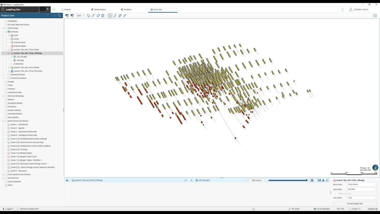
I would just demo quickly how to do a grouped lithology.

[00:15:01.320]
So we’ll right click on the lithology table,

[00:15:04.310]
create a new column grouped lithologies.

[00:15:08.680]
The base column will be our lithology that we’ve imported,

[00:15:14.290]
and I’ll call this one Lith_Grouped.

[00:15:18.690]
We can manually group these codes or we can also group them.

[00:15:24.410]
For this example, I’m just going to auto group

[00:15:26.730]
based on the first letter of each code.

[00:15:31.730]
That’s going to pop all of those codes into these groups

[00:15:35.810]
on the right hand side here.

[00:15:40.300]
I can see all of my C codes, this is my colluvium,

[00:15:46.310]
the F codes are felsics,

[00:15:51.740]
the L codes are the regolith codes,

[00:15:58.150]
our M codes are mafics, and our S codes are our sediments.

[00:16:04.810]
So our CIF,

[00:16:05.750]
which is our mineralized lithology in this project.

[00:16:09.850]
So I’ll just call this one seds,

[00:16:13.280]
make the mafics green

[00:16:28.920]
and click okay.

[00:16:31.612]
We take a look at that table now in the scene view.

[00:16:39.335]
I can see that we’re looking at our Lith_Grouped

[00:16:41.620]
in the dropdown here, and we can also jump back

[00:16:44.350]
and look at the imported lithology.

[00:16:47.360]
So we’ve greatly simplified our lith codes

[00:16:50.900]
using that grouping,

[00:16:52.890]
and we can really easily see now where our seds are sitting,

[00:16:57.220]
they’ve been grouped together,

[00:17:00.360]
and we’ve made it a lot cleaner for modeling

[00:17:02.500]
if we want to model our base of transported

[00:17:05.600]
and our regolith.

[00:17:08.380]
The next tool we’ll have a quick look at in Leapfrog

[00:17:13.530]
is the interval selection tool.

[00:17:17.100]
This is a really powerful tool in Leapfrog.

[00:17:19.550]
It’s commonly used as it gives you significant control

[00:17:22.560]
over the intervals you’re use to build your models.

[00:17:26.090]
If you’re building your geological models

[00:17:27.810]
based on drillhole data,

[00:17:29.420]
we recommend always basing your geological model

[00:17:32.020]
on an interval selection column

[00:17:34.270]
rather than the original imported column.

[00:17:37.820]
This provides maximum flexibility

[00:17:40.050]
as you progress with your modeling.

[00:17:43.720]
I’ll create an interval selection column.

[00:17:46.260]
So bring our lithology back on,

[00:17:54.150]
right click on the lithology table,

[00:17:56.360]
create a new column, and choose interval selection.

[00:18:01.290]
There are a couple of options here.

[00:18:03.690]
We can choose to have a base column of none.

[00:18:07.140]
And this means you need to build

[00:18:08.530]
your interval selection column from scratch.

[00:18:10.990]
It does give you ultimate control

[00:18:12.570]
over the contents of this column,

[00:18:14.920]
but you might end up with a lot of flicking back and forth

[00:18:17.500]
and the shape list to see your raw data.

[00:18:21.730]
The other option is to choose

[00:18:23.150]
one of the existing lithologies or categories

[00:18:26.900]
as the base column.

[00:18:28.900]
So for example, we can choose our Lith_Grouped

[00:18:31.810]
as the base column for this interval selection,

[00:18:34.730]
and it will copy all of the intervals

[00:18:36.630]
over from the existing table

[00:18:39.050]
and then you can change the codes as needed for modeling.

[00:18:43.150]
This approach is useful

[00:18:44.430]
if you only need to make minor modifications

[00:18:47.000]
to the imported unit codes,

[00:18:49.210]
or for example, your modeling based on grade

[00:18:52.410]
using a category from numeric column.

[00:18:55.920]
I prefer using this option

[00:18:57.490]
as it requires less flicking back and forth,

[00:18:59.650]
and all of the intervals are already populated

[00:19:01.930]
ready for interpretation.

[00:19:03.810]
But ultimately how you set up your tables

[00:19:06.060]
and work flows is up to you and your company,

[00:19:09.200]
and it will be quite project specific.

[00:19:12.560]
In this case, we’ll set the Lith_Grouped as the base column

[00:19:16.190]
and I’ll call this Lith_Selection.

[00:19:21.540]
And this now gives us the option to split out

[00:19:25.390]
any of our grouped lithologies

[00:19:27.340]
and assign them to a new category.

[00:19:30.410]
So for example, here, we can split out these seds

[00:19:35.620]
into different units if we want to for modeling.

[00:19:40.860]
The next column type that we’ll look at quickly

[00:19:43.900]
is the split lithologies tool.

[00:19:47.020]
It’s one that I don’t use very often

[00:19:49.050]
as it’s more limited than the interval selection.

[00:19:52.520]
With this split lithologies,

[00:19:55.980]
you can create new units from a single code

[00:20:00.080]
by selecting from intervals displayed in the scene.

[00:20:03.490]
The difference between the interval selection tool

[00:20:06.010]
and the split lithologies tool is that

[00:20:08.296]
with the split lithologies,

[00:20:10.420]
you’re limited to selecting intervals

[00:20:12.780]
only from a single lithology,

[00:20:14.387]
and I’ll show you how that works here.

[00:20:21.690]
So here, for example, I’ll select my CIF

[00:20:24.890]
as the main unit that I’m looking at,

[00:20:27.720]
and I’m limited to only selecting CIF interval.

[00:20:32.930]
So for example, if there is any mislogging

[00:20:36.210]
and I wanted to select an interval inside the CIF

[00:20:41.580]
to assign it to CIF,

[00:20:42.710]
I can’t do that with the split lithologies,

[00:20:45.430]
but I could with the interval tool.

[00:20:50.360]
The next kind of created column we’ll take a quick look at

[00:20:54.180]
within Leapfrog is the drillhole correlation.

[00:20:59.060]
With the drillhole correlation tool,

[00:21:01.200]
you can view and compare selected drillholes in a 2D view,

[00:21:05.390]
you can then create new interpretation tables

[00:21:07.940]
in which you can assign and adjust intervals

[00:21:10.440]
and create new intervals as needed.

[00:21:14.520]
Interpretation tables are like any other interval table

[00:21:17.950]
in a project, and can be used to create models.

[00:21:21.210]
You can also save and export correlation set layouts

[00:21:25.340]
and styles that can then be used

[00:21:27.950]
in other Leapfrog Geo projects.

[00:21:31.250]
Some useful applications of the drillhole correlation tool

[00:21:34.430]
include for geological modeling

[00:21:36.700]
of consistent strap sequences

[00:21:39.200]
or for comparing economic composites between holes.

[00:21:43.970]
I’ll set up a drillhole correlation set now.

[00:21:55.817]
And so I’ll pick the collars back in the scene view

[00:21:58.740]
that I’m interested in looking at,

[00:22:07.780]
and we can drag across any of the columns

[00:22:12.130]
that we have here in the project tree.

[00:22:14.100]
So for example, our Lith_Group

[00:22:17.000]
versus our original lithology, we can compare here,

[00:22:27.670]
and we can add in new interpretation tables.

[00:22:33.310]
So I’ll set my source column,

[00:22:36.330]
I can populate an empty table,

[00:22:39.180]
kind of like setting the base lithology to none

[00:22:41.810]
for an interval selection,

[00:22:43.850]
or I can populate all intervals to start off with

[00:22:46.700]
and they can then be adjusted.

[00:22:52.810]
So here I’ve started off with the same intervals

[00:22:56.820]
as the Lith_Grouped,

[00:22:58.820]
but now I have the option to adjust here into day

[00:23:03.370]
and make changes

[00:23:04.730]
based on other information that I might have.

[00:23:10.470]
I’ll save that.

[00:23:11.690]
And we’ve now got this new interpretation table

[00:23:15.040]
in the project tree that can be used to model.

[00:23:18.760]
The next tool we’ll take a quick look at

[00:23:20.810]
is the overlaid lithology tool.

[00:23:23.310]
So this lets you combine two columns

[00:23:25.820]
to create one new column.

[00:23:28.240]
There’s a primary column.

[00:23:29.620]
So this is the column that you wish to have precedence

[00:23:32.960]
and then a fallback column.

[00:23:34.540]
So data in that fallback column will only be used

[00:23:37.540]
when no data is available from the primary column.

[00:23:41.890]
An example here might be where we’ve logged oxidized

[00:23:45.460]
and transitional material in one column,

[00:23:47.540]
but we haven’t logged fresh.

[00:23:49.620]
So we may want to combine

[00:23:51.530]
that oxidized and transitional material

[00:23:54.070]
with our logged fresh cards.

[00:23:57.090]
So I’ll set that up quickly.

[00:23:58.620]
I’ll bring in our additional weathering column,

[00:24:13.890]
and we’ll set up the overlaid lithology.

[00:24:19.070]
So here we can set our weathering as the primary column

[00:24:22.200]
and our grouped lithology as the fallback column.

[00:24:27.020]
And then it will only populate our grouped lith

[00:24:29.460]
where there are no weathering codes.

[00:24:31.460]
And we can assume that

[00:24:32.850]
all of the oxidized and transitional material

[00:24:36.270]
will be populated from the weathered column,

[00:24:38.280]
and then everywhere that we have our fallback column

[00:24:40.880]
is fresh.

[00:24:54.030]
And we’ll take a look at that

[00:24:55.740]
on our drillhole correlation sets as well.

[00:25:03.530]
So you can see our combined column here.

[00:25:05.510]
So everywhere where we’ve got data in our weathering column,

[00:25:11.300]
we’ve populated as the primary column

[00:25:14.390]
in the overlaid lithology,

[00:25:16.370]
and then where we don’t have data,

[00:25:18.100]
we’ve got our grouped lithology.

[00:25:25.330]
The next type of column we’ll have a look at

[00:25:27.770]
is the category column from numeric data.

[00:25:31.150]
And this is used when you’ve got your numeric data

[00:25:33.450]
that you wish to turn into categories or bins

[00:25:36.510]
so that you can use that with the lithology

[00:25:39.060]
and category modeling tools within Leapfrog.

[00:25:42.570]
This data can then be interval selected and used as the base

[00:25:46.190]
for a domain model or a geological model.

[00:25:49.560]
An example of this is for narrow vein modeling

[00:25:52.750]
in gold deposits.

[00:25:54.410]
The grade and logging are often combined together

[00:25:57.870]
to determine domain boundaries that we may need to make sure

[00:26:01.520]
that we’re selecting based on the assay data.

[00:26:07.100]
I’ll quickly set up a category from numeric.

[00:26:13.320]
So we’ve got our raw assay data here

[00:26:22.490]
with a continuous color map.

[00:26:25.700]
To set up the category from numeric,

[00:26:27.620]
we’ll right click on the assay table

[00:26:30.020]
and create a new column category from numeric.

[00:26:34.180]
The base column will be gold

[00:26:36.120]
and we’ll call this one Au_cat.

[00:26:39.860]
We can now add in different categories.

[00:26:42.760]
So my lowest category might be a 0.05

[00:26:58.600]
then we’ll have a 0.5, a one,

[00:27:08.820]
a three, and we’d put a 10 in there as well.

[00:27:16.070]
We need to adjust these names

[00:27:30.570]
and make sure that you’ve got the symbol

[00:27:33.040]
the way that you want it to be.

[00:27:34.440]
So decide if the assay lands exactly on the number,

[00:27:39.480]
whether you want to end the bin above or below.

[00:27:54.230]
I will set the colors up here and click okay.

[00:27:59.120]
Now in that assay table, we can drop down to the Au_cat

[00:28:02.650]
rather than that raw gold data

[00:28:06.410]
with the continuous color map.

[00:28:08.560]
And we’ve binned all of our assays into these grade bin.

[00:28:16.710]
This can be used as the base column

[00:28:18.950]
for an interval selection if we want to,

[00:28:21.690]
and we can then select based on our Au_cat intervals.

[00:28:28.570]
Next up, we’ll take a look at creating new columns

[00:28:31.500]
in the composites folder.

[00:28:33.510]
So we can create category composites, majority composites,

[00:28:37.210]
numeric composites, or economic composites here,

[00:28:40.480]
and we’ll quickly run through the functionality

[00:28:42.530]
for each of these types.

[00:28:45.700]
The category comps can be used

[00:28:50.700]
if unit lith boundaries are poorly defined.

[00:28:53.750]
For example, if there are small fragments

[00:28:55.720]
of other lithologies within the lith of interest,

[00:28:59.480]
the category comp tends to smooth these out.

[00:29:04.250]
So we can composite the drillhole data directly here

[00:29:07.170]
using the category comp functionality.

[00:29:10.070]
This creates a new interval table

[00:29:11.870]
that can be used to build models,

[00:29:13.750]
and changes made to the table

[00:29:15.400]
will be reflected in all models based on that table.

[00:29:19.280]
So we’ll set up a new category comp from the Lith_Grouped.

[00:29:26.070]
Our primary unit of interest in this model is the seds.

[00:29:30.850]
And in this case,

[00:29:31.920]
we’ll ignore the colluvium, felsics, and regolith,

[00:29:35.210]
and we’ll just look at comping small segments of mafic

[00:29:39.570]
that are caught within the seds.

[00:29:42.520]
So this is where we set that length.

[00:29:44.910]
So we can filter these exterior segments,

[00:29:47.740]
let’s say shorter than two meters,

[00:29:52.020]
and that will simplify our seds for modeling

[00:29:56.480]
if we’re happy to include two meters of mafic

[00:29:59.340]
inside our seds.

[00:30:00.990]
So again, it really depends

[00:30:02.410]
on what you’re building the model for and why.

[00:30:06.340]
So the settings here will be dependent on that.

[00:30:15.080]
So dragging that into the scene view,

[00:30:16.900]
we can see

[00:30:20.097]
that we’ve ignored the segments in gray,

[00:30:22.980]
primary segments in red, and the exterior segments in blue.

[00:30:28.740]
And we can have a look using the drillhole correlation

[00:30:31.970]
and compare our original grouped lithology

[00:30:35.250]
to the category comp.

[00:30:36.900]
So I’ll just set up and grab a couple of colors there.

[00:30:56.720]
We’ll bring on our comp and we’ll bring on our Lith_Grouped.

[00:31:06.470]
So we can see here in hole SKA350,

[00:31:12.990]
in our Lith_Grouped we had a small interval of mafics

[00:31:17.350]
and that has now been composited into our primary lithology.

[00:31:22.820]
The second option for compositing these points

[00:31:25.790]
is rather than doing it directly on the drillhole

[00:31:29.750]
is to change the settings in the intrusion surfaces

[00:31:32.710]
and the geological model.

[00:31:34.950]
We have very similar settings

[00:31:37.040]
that can be changed at that stage,

[00:31:39.510]
and I prefer to use the second option

[00:31:41.510]
in the surfacing settings

[00:31:42.670]
as it keeps the underlying data as is,

[00:31:46.100]
but adjust the input points building that intrusion

[00:31:49.290]
based on the compositing parameters that you set up.

[00:31:52.780]
This is covered in our advanced surface editing training

[00:31:55.720]
and also in a previous webinar.

[00:32:02.050]
Using the majority composites tool,

[00:32:04.930]
we can comp category data into integral lengths

[00:32:08.870]
from another table or into fixed interval lengths.

[00:32:12.110]
So we’ll take a look at that.

[00:32:14.920]
So a new majority composite, we can set a fixed length,

[00:32:19.290]
or we might want to set our assay length.

[00:32:23.220]
We may want to comp our grouped lithology

[00:32:26.360]
based on our assay intervals.

[00:32:29.630]
This is really useful for comparing

[00:32:31.410]
those lith and assay intervals as the intervals,

[00:32:34.793]
the from’s and the to’s from the assay table

[00:32:36.980]
will be applied to the category column

[00:32:39.910]
to produce a new column with those shorter intervals.

[00:32:44.560]
The majority comp can then be used to create

[00:32:47.630]
or used in a merged table

[00:32:50.160]
containing both assay and lithology data.

[00:32:53.310]
And the key benefits of this workflow

[00:32:55.610]
is that the merge table will not split the assays,

[00:32:59.090]
though those assay intervals will still be maintained

[00:33:02.250]
even if the lith intervals don’t align.

[00:33:06.950]
So I’ll set up one of those.

[00:33:12.200]
And if we open up that majority comp,

[00:33:15.270]
we can say that for each interval,

[00:33:17.570]
we have a Lith_Grouped code.

[00:33:26.290]
The numeric comp tool will take

[00:33:29.760]
unevenly spaced drillhole data

[00:33:31.660]
and turn it into regularly spaced data,

[00:33:33.730]
which can then be used in an interpolation or an estimation.

[00:33:38.710]
The compositing parameters can be applied

[00:33:41.420]
to the entire drillhole, or just within a subset of codes.

[00:33:46.930]
For example, we might want to just compare gold values

[00:33:49.780]
within the CIF.

[00:33:52.380]
So here we can set our base column to our Lith_Grouped

[00:33:59.090]
and just comp the seds to let’s do a two meter interval.

[00:34:07.400]
There are some other options here

[00:34:08.930]
for residual end length and minimum coverage.

[00:34:13.170]
If you’d like some more information about these,

[00:34:15.240]
please get in touch with us,

[00:34:17.460]
as the minimum coverage can have quite a large impact,

[00:34:21.350]
particularly if you have missing intervals

[00:34:23.270]
and missing samples.

[00:34:26.580]
We’ll choose our output column there.

[00:34:28.120]
So we’ll choose the Au and click okay.

[00:34:40.270]
And we’ve got our numeric comp now in the scene view.

[00:34:46.460]
You can see we have only comped that data

[00:34:48.930]
that fell within the CIF unit.

[00:34:54.390]
The final type of composite we can create

[00:34:56.900]
in Leapfrog is an economic composite.

[00:34:59.860]
The economic comp classifies assay data

[00:35:02.520]
into either/or, or waste,

[00:35:05.390]
and can take into account grade thresholds,

[00:35:07.840]
mining dimensions, and allowable internal dilution.

[00:35:11.880]
The result is an interval table

[00:35:13.670]
with a column of all waste category data,

[00:35:17.000]
a column of composited interval values,

[00:35:19.590]
plus some additional columns showing the lengths,

[00:35:22.750]
linear grade, included dilution length,

[00:35:25.990]
included dilution grade, and the percentage of the comp

[00:35:29.180]
that’s based on missing interval data.

[00:35:32.810]
There’s a free training module on My Seequent,

[00:35:35.510]
which runs through this in more detail

[00:35:38.120]
and also a webinar on our website.

[00:35:41.240]
I’ll create an economic comp here

[00:35:48.300]
using gold values,

[00:35:51.140]
and we’ll set a cutoff grade of two

[00:35:54.070]
and on a minimum or comp length of three.

[00:35:57.060]
We’ll just set a really simple one now for demo purposes.

[00:36:08.102]
You can see in the scene view now we have our drillholes.

[00:36:16.183]
All of the intervals have either been classified

[00:36:18.563]
as ore in red or waste in blue.

[00:36:23.141]
It can be quite handy to use the drillhole correlation

[00:36:26.760]
to compare how we’ve comped across different drillholes

[00:36:30.390]
on the same line.

[00:36:32.520]
So I’ll set up a new drillhole sed quickly.

[00:36:44.017]
So I’ll compare a few holes here.

[00:36:48.970]
Can bring across the status and the grade.

[00:37:01.085]
We can see across those holes,

[00:37:03.070]
we’ve actually only got ore based on those parameters

[00:37:05.970]
in every second hole here.

[00:37:10.900]
Another way to create new columns in Leapfrog

[00:37:14.390]
is by using the calculations on our drillhole data.

[00:37:18.690]
So these calculations might be metal equivalencies

[00:37:21.510]
or elemental ratios that can then be used

[00:37:23.840]
in downstream modeling or interpretation.

[00:37:27.270]
The calculations can be found by right clicking

[00:37:30.960]
on any of the drillhole tables and going to calculations.

[00:37:35.240]
We can then set up a variable, a numeric calculation,

[00:37:39.510]
or a category calculation using any of these existing items

[00:37:44.450]
and the syntax and functions

[00:37:46.080]
found here on the right hand side.

[00:37:51.540]
And finally, the last way to create new columns

[00:37:56.090]
within Leapfrog is by back flagging drillhole data

[00:37:58.870]
with an existing model.

[00:38:01.260]
So this will flag our domain model

[00:38:03.690]
back against our drillholes,

[00:38:05.190]
and create new tables and columns within Leapfrog.

[00:38:12.290]
Once we’ve set up all of these columns and tables

[00:38:15.890]
that we need for our interpretation,

[00:38:18.350]
sometimes maybe we might want to merge that data together.

[00:38:21.840]
That’s where the merged table functionality comes in.

[00:38:30.920]
The merge table functionality simply brings together columns

[00:38:34.160]
from multiple tables into a single table,

[00:38:37.060]
and there are many applications for this within Leapfrog,

[00:38:40.170]
including for these two reasons here.

[00:38:42.770]
So one would be to allow

[00:38:44.280]
for more flexible interval selection.

[00:38:48.070]
And the other reason here that we’ve got

[00:38:50.230]
is to combine numeric and categorical data

[00:38:53.380]
into a single table

[00:38:54.700]
for the purpose of domain-specific statistical analysis

[00:38:58.110]
of that data.

[00:39:00.930]
The merge table preserves all intervals

[00:39:03.470]
from all tables being merged,

[00:39:05.800]
which depending on the logging practices

[00:39:07.890]
that you’ve got on your site

[00:39:09.620]
may result in assay intervals being split.

[00:39:13.210]
To preserve the assay intervals and create a merge table

[00:39:16.380]
containing assay and lithology data

[00:39:18.470]
without splitting those intervals,

[00:39:20.870]
start by creating a majority comp table first,

[00:39:24.060]
and then using that majority comp

[00:39:25.810]
to merge in with your assays.

[00:39:31.430]
An important note here is that

[00:39:32.910]
if you build an interval selection column

[00:39:35.790]
from a merge table, preserving the from and to intervals

[00:39:40.010]
in that merge table is very important.

[00:39:43.170]
If the from or to values in the merge table get adjusted,

[00:39:47.550]
the interval selection coding for those rows

[00:39:49.900]
will be removed and you’ll lose those selection codes

[00:39:52.920]
in the interval selection.

[00:39:55.360]
Merge tables are dynamically linked

[00:39:57.040]
back to their source tables.

[00:39:58.770]
So a change in the interval length in the source table.

[00:40:02.650]
So for example, if the hole gets relogging

[00:40:05.010]
and then reloaded with different from’s and to’s,

[00:40:08.240]
this would lead to a change of interval length

[00:40:10.400]
in the merge table,

[00:40:11.850]
and result in the loss of some of your interval selections.

[00:40:15.660]
So be careful with this.

[00:40:20.470]
We have some really great charts

[00:40:22.150]
and workflow documents here on merge tables.

[00:40:25.090]
If you would like a copy of these,

[00:40:27.610]
please get in touch with us after the webinar

[00:40:29.790]
and we can send them through.

[00:40:32.290]
So this one here, it’s just a brief workflow chart

[00:40:37.480]
on merge tables asking that why

[00:40:40.770]
and when you should merge tables,

[00:40:42.340]
depending on what you’re planning to use them for.

[00:40:45.100]
And there’s some information in here

[00:40:46.740]
about whether you should build the merge table

[00:40:49.480]
before performing your interval selection and modeling

[00:40:52.010]
or afterwards

[00:40:52.910]
depending on what workflow you’re trying to do.

[00:40:56.651]
And we’ve got a document for workflow 1 as well

[00:40:59.440]
that runs through creating that majority comp first

[00:41:03.070]
and then merging that with your assays

[00:41:06.190]
so that you keep those assay interval lengths.

[00:41:10.590]
So, yeah, please get in touch

[00:41:11.640]
if you’d like a copy of these and we’ll send them out.

[00:41:18.930]
And finally, once we’ve validated and interpreted our data,

[00:41:24.280]
merge tables, if we need to set up interval selections,

[00:41:28.090]
we can choose a base lithology column

[00:41:30.220]
for our geological model or domain model.

[00:41:34.940]
An important thing to know is that

[00:41:36.360]
once the base lith column has been set,

[00:41:38.590]
it cannot be changed, so choose carefully.

[00:41:43.840]
Any of the column types that we’ve discussed so far

[00:41:46.660]
or any of those category or lithology column types

[00:41:49.270]
can be used as the base column.

[00:41:52.000]
So this might be an interval selection

[00:41:53.580]
on a grouped lithology or an interval selection

[00:41:56.760]
on a category from numeric column,

[00:41:58.650]
or perhaps even the status column from an economic comp.

[00:42:02.190]
They can all be used as the base column

[00:42:04.100]
for your geology model.

[00:42:06.500]
The other option we have is to have a base column of none.

[00:42:10.030]
I’ll just bring up the new geological model window.

[00:42:16.680]
So here we can have a base column of none if we want to.

[00:42:21.150]
So when you select this,

[00:42:22.510]
the point is to not link the model to any source column.

[00:42:25.730]
So this means you’re free to remove source columns

[00:42:27.960]
if needed, and you can model

[00:42:29.960]
from multiple different data sources.

[00:42:32.620]
This can be a good option if you’re creating a model

[00:42:35.640]
from information other than drillhole data.

[00:42:38.820]
So for example, GIS lines, polylines,

[00:42:42.150]
existing surfaces or structural data,

[00:42:44.660]
then you could select none.

[00:42:50.630]
A query filter can also be applied at this stage

[00:42:53.890]
when setting up the geology model.

[00:42:56.160]
So for example, we might wish to filter out those holes

[00:42:59.110]
that we classified earlier as low confidence.

[00:43:02.470]
So, I’ll just quickly write the query filter for that.

[00:43:14.870]
So I’ve build my query, and say that I want my confidence

[00:43:19.540]
to only be high or medium.

[00:43:33.780]
I’ll set my base lithology column to my Lith_Selection

[00:43:37.930]
so that I’ve got maximum flexibility,

[00:43:40.510]
and I’ll apply my query filter.

[00:43:43.380]
Now we’re ready to go and start modeling.

[00:43:47.510]
Thank you for attending this webinar today.

[00:43:49.960]
We hope that this has been a helpful guide

[00:43:53.500]
to understanding drillhole data in Leapfrog,

[00:43:56.240]
and assists with importing, validating,

[00:43:58.910]
and interpreting data to get ready for modeling.

[00:44:07.010]
As always, if you need any help,

[00:44:09.160]
please get in touch with your Seequent support team

[00:44:11.800]
at [email protected].

[00:44:14.830]
And we have great resources on our website,

[00:44:17.410]
in the My Seequent Learning,

[00:44:19.510]
and we run training and project assistance.

[00:44:22.520]
So again, please contact your local team

[00:44:24.740]
if you need any help with training and project assistance.

[00:44:28.650]
Thank you.