


Introduction
There are many problems in geotechnical engineering that involve a coupling between climatic conditions and the thermal response within the ground. These types of problems are often termed in the literature as land-climate interaction or soil-vegetation-atmosphere (SVA) interaction problems. Some examples include the protection of permafrost in northern regions, the design of near-surface geothermal energy systems, design and construction of frozen capillary barrier cover systems, and the design of foundation insulation in cold climate regions. In these cases, the thermal response within the ground is highly dependent on the atmospheric conditions, which in turn, are a function of the land surface conditions.
Engineering problems of this nature require a description of the energy transfers between the ground surface and the atmosphere, termed the surface energy balance. The global objective of this example is to describe and demonstrate the use of the surface energy balance (SEB) boundary condition implemented in TEMP/W. The specific objectives of this example include:
1. Highlighting the key climate and material inputs;
2. Demonstrating the insulating capacity of the snow pack during winter conditions on the
thermal response of the ground; and,
3. Demonstrate the numerical stability of the TEMP/W implementation for an SEB boundary
condition.
Background
The amount of energy delivered to the earth’s surface from the atmosphere is the difference between the net shortwave and net longwave radiation (i.e. net radiation). This energy is utilized by a number of processes at the land surface such as evapotranspiration, sublimation, changing the air temperature, and changing the soil temperature (heating or cooling the ground). The energy conservation statement at the land surface can be written as:
(𝑞𝑛𝑠 ‒ 𝑞𝑛𝑙) = 𝑞ℎ + 𝑞𝑙 + 𝑞g
where
𝑞𝑛𝑠 Net solar (shortwave) radiation [MJ m-2 day-1]
𝑞𝑛𝑙 Net terrestrial (longwave) radiation [MJ m-2 day-1]
(𝑞𝑛𝑠 ‒ 𝑞𝑛𝑙) Net radiation [MJ m-2 day-1]
𝑞ℎ Sensible heat flux [MJ m-2 day-1]
𝑞𝑙
Latent heat flux [MJ m-2 day-1]
𝑞𝑔 Ground heat flux [MJ m-2 day-1]
(Equation 1)
All of the energy terms in this equation are flux rates, defined as the amount of energy rate per unit area. The sign convention of Sellers (1968) is adopted such that net radiation is positive downwards (toward the surface); latent and sensible heat fluxes are positive upwards (away from the surface), and ground heat flux is positive downward (into the ground). The equation states that all energy received at the earth’s surface must be used to warm or cool the air above the ground surface (sensible heat flux), evaporate water (latent heat flux), or warm or cool the ground (ground heat flux). Details of the individual energy flux terms are presented in the Engineering Book.
The thermal response within the domain is controlled primarily by the ground heat flux in an analysis involving climate interaction. A positive ground heat flux implies energy input into the ground, while a negative ground heat flux indicates energy extraction. Equation 1 is therefore solved for the
ground heat flux as:
𝑞𝑔 = (𝑞𝑛𝑠 ‒ 𝑞𝑛𝑙) ‒ 𝑞ℎ‒ 𝑞𝑙
(Equation 2)
The ground heat flux is solved as the residual of the energy balance equation and applied as the boundary condition on the finite element domain. The surface energy balance equation can be re-written to accommodate the presence of snow during the winter months as:
𝑞𝑠𝑛𝑜𝑤 = 𝑞𝑔 = (𝑞𝑛𝑠 ‒ 𝑞𝑛𝑙) ‒ 𝑞ℎ‒ 𝑞𝑙
(Equation 3)
where the energy flux through the snow is assumed equal to , which infers that the snow 𝑞𝑠𝑛𝑜𝑤 𝑞𝑔 does not have the capacity to store energy. It should be noted that the application of a flux boundary condition in a finite element analysis can often lead to numerical instability. The instantaneous flux rate calculated at the beginning of a time step can result in an excessive amount of energy being extracted or injected into the domain. In turn, the temperature of the ground is under or overestimated, resulting in a reversal of the flux rate on the subsequent time step. Eventually, the analysis becomes prone to numerical oscillation. The SEB boundary condition is implemented within TEMP/W in such a manner so as to prevent this oscillation from occurring; thereby ensuring a numerically stable solution even with larger time steps.
Numerical Experiment
TEMP/W was used to model a case study presented by Hwang (1976). The objective of this example is to demonstrate the process of modeling a surface energy balance problem. It should be noted that TEMP/W implements different equations for surface energy balance components than those presented by Hwang (1976), particularly for calculating sensible heat flux and net longwave radiation. Accordingly, the results will differ from the publication and no attempt was made to calibrate the model or replicate the original results.
The study site was located in northern Canada at Normal Wells, Northwest Territories (latitude 65.2°). The major stratigraphic units comprised peat, silt, and till overlying a shale unit. The thermal properties of each unit were modelled using a simplified thermal model. The simplified model assumes a constant thermal conductivity and volumetric heat capacity for the frozen and unfrozen conditions. The in situ volumetric water content for each unit was assumed to be 0.35.
The climate data was scaled from the figures presented by Hwang (1976), entered into a spreadsheet, converted into the appropriate units, and then pasted into the boundary functions (see GSZ file). The summer and winter albedo was assumed to 0.15 and 0.50, respectively. The snow conductivity was set to 10.45 kJ/m/°C. A vegetation height of 0.001 m was used to model a bare ground condition.
Convergence was based on two significant digits or a minimum difference of 0.1°C for two successive iterations. This is a fairly relaxed tolerance for a surface energy balance problem; however, the one dimensional nature of the problem helps improve convergence.
Results and Discussion
Figure 1 compares the simulated ground surface temperature response with the values presented by Hwang (1976). Note that the associated GeoStudio file was only solved for the first 30 days to minimize file size. The analysis was solved using time steps of 2 hours, 12 hours, and 24 hours. The TEMP/W results capture the trends of Hwang’s predictions for all time step sizes. The ground surface temperature varies between – 10°C and – 15°C during the winter, despite the air temperature dropping below – 30°C (Figure 2). This is due to the insulating capacity of the snowpack, which dampens the ground heat flux. It should be noted that in this example diurnal fluctuations in ground temperature are not captured due to the resolution of the climate data. The incoming shortwave radiation in particular was assumed constant over approximately 15 day intervals.
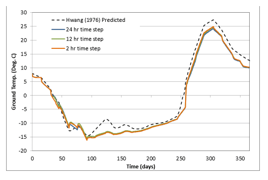
Figure 1. Ground temperature response for three different time steps.
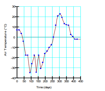
Figure 2. Air temperature function.
Figure 3 compares the simulated ground surface temperature-time history to that at 0.3 m and 1.0 m depths. The cooling and warming trends are delayed and dampened at depth relative to the response at the ground surface. The temperature at 1 m below ground surface hovers around 0C as latent heat is released from the soil between day 50 and day 75. The delay at 1 m depth is more pronounced than at 0.3 m depth, which occurs just before day 50, because the ground heat flux is nearly constant and smaller during this time (Figure 4). Note that the ground temperatures are nearly constant and do not exhibit fluctuations from about Day 100 to Day 250, due primarily to the increased snowpack thickness. This is also reflected in the lower ground heat fluxes during this time.
On day 250, the ground heat fluxes begin to increase rapidly, which in turn cause the ground temperatures to rise.
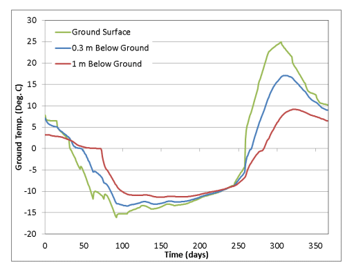
Figure 3. Ground temperature response at 0.3 m and 1 m below ground.
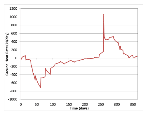
Figure 4. Ground heat flux verses time.
Summary and Conclusions
The surface energy balance boundary condition in TEMP/W can be used to model the coupled response between the ground and atmosphere. The boundary condition requires a number of climatic inputs including: air temperature, wind speed, radiation, vegetation height, evaporation height, and snow depth. These inputs are then used to calculate the key components of a surface energy balance, which is ultimately used to compute the ground heat flux boundary condition.
A case history presented by Hwang (1976) is analyzed in this example. The results compare favourably to the predictions made by Hwang despite the fact that the implementations are different and no attempt was made to calibrate the model. Moreover, the analysis demonstrates the insulating effects of snow as the ground temperature fluctuations are dampened, even though the air temperature changes dramatically over the winter months. Finally, the SEB boundary condition implementation in TEMP/W is numerically stable even when large time steps are used.
References
Hwang, C.T. 1976. Predictions and observations on the behaviour of a warm gas pipeline on permafrost. Canadian Geotechnical Journal, 13: 452 – 480. Sellers, W.D. 1965. Physical Climatology. University of Chicago Press. Chicago, Illinois.