


Introduction
There are three basic boundary conditions for contaminant transport: 1) specified concentration (Dirichlet); 2) specified dispersive flux (Neumann); and, 3) specified dispersive and advective flux (Cauchy). In many cases, these boundary conditions are sufficient and easily defined. For example, a contaminant source could be specified using either the Dirichlet (constant concentration) or Cauchy (constant mass flux) type boundary condition. In transport analyses, however, the plume often reaches the far-field boundary, making the aforementioned boundary conditions incorrect. Frind (1988) formulated a free exit mass flux boundary condition that allows mass to exit by both advection and dispersion. The boundary condition is a Cauchy type that responds to the changing concentration at the boundary.
The objectives of this example are to: 1) demonstrate the use of the constant and source concentration boundary conditions; 2) demonstrate the use of the free exit and mass rate exit boundary conditions; and, 3) compare the results from CTRAN/W to a closed-form solution of the advection-dispersion equation.
Background
Frind (1988) presents the following closed-form analytical solution to the advection-dispersion equation for a one-dimensional semi-infinite medium with a Cauchy boundary condition:
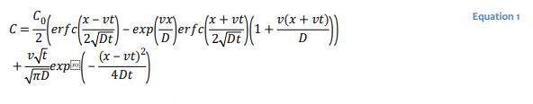
where 𝐶 is the concentration, 𝐶0 is the specified concentration in the source boundary, 𝐷 is the hydrodynamic dispersion coefficient, 𝑣 is the average linear velocity, 𝑡 is the elapsed time, 𝑥 is the distance from the source boundary, and 𝑒𝑟𝑓𝑐 is the complementary error function.
Numerical Simulation
Figure 1 presents the one-dimensional model domain. The GeoStudio Project file includes a steady-state water transfer analysis and four transient solute transfer analyses (Figure 2). The advection-dispersion physical process is selected in the physics tab (Figure 3) for all transport analyses. Case 1 and 2 compare the options for defining the source boundary condition: a constant concentration and a source concentration. The last two analyses compare two of the boundary conditions available for defining the mass exit boundary condition: free exit mass flux and the zero mass flux.
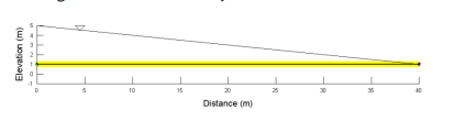
Figure 1. Problem configuration.
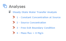
Figure 2. Analyses tree for the Project file.
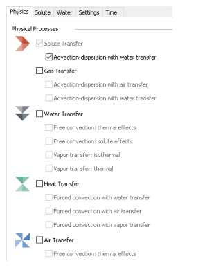
Figure 3. Physics tab for the solute transfer analyses.
The hydraulic properties are characterized using the Saturated-Only material model. The saturated hydraulic conductivity and volumetric water content were assumed to be of 0.5 m/sec and 0.5, respectively. Constant total head boundary conditions of 5 m and 1 m were specified on the left and right sides of the domain, respectively.
A total head loss (∆ℎ) of 4 m occurs over the 40 m column, making the hydraulic gradient (𝑖) equal to 0.1 m/m. The water flux, or Darcy velocity, through the column is therefore 𝑞 = 0.5(0.1) = 0.05m3/s/m2. The interstitial velocity (𝑣) is calculated as 𝑣 = 𝑞/𝜃 = 0.05/0.5 = 0.1 m/s.
For all of the solute transport analyses, the material properties are defined using the Advection-Dispersion material model. The dispersivity a is specified as 4 m and diffusion is assumed inoperative, which makes the coefficient of hydrodynamic dispersion equal to that of mechanical dispersion m2 𝐷 = 𝛼𝑣 = 0.4 /sec. Decay and adsorption are not included in the analyses. The material is activated with a concentration of 0 Mg/m3 at the start of each analysis.
In Case 1, a constant concentration of 1 Mg/m3 is specified at the left boundary. The right boundary is unspecified. For the remaining three cases, the left boundary is defined using the source boundary condition (𝑞 × 𝐶 ) set to 1 Mg/m3 . This boundary condition can be used to represent a contaminated body of water that is acting as a source to the soil. As such, the actual concentration at the boundary depends on both the water rate and fluid concentration. The right boundary is also unspecified in Case 2 for comparison to Case 1.
Case 3 uses the free exit mass flux boundary condition on the right edge, which allows mass to exit via dispersion and advection. In contrast, the boundary is specified as a zero mass rate in Case 4 (𝑄𝑚 = 0 𝑀𝑔/𝑠𝑒𝑐 ), which implies that mass cannot leave the domain. This type of boundary condition would be required to model, for example, the salinization that develops in ground water discharge locations.
Applying a zero mass rate boundary condition to the right edge may seem counter-intuitive. In most finite element formulations, the net flow rate at every node is implicitly zero unless a boundary condition has been specified. For example, the water rate at every node is zero in a SEEP/W analysis. However, the natural boundary condition for the CTRAN/W formulation is the divergence of the dispersive mass rate, not the total mass rate. As such, a total mass flux or total mass rate of zero must be specified to ensure that both advective and dispersive flux is zero.
Results and Discussion
Figure 4 presents the concentration distribution at each time step for Case 1. The concentration at the left boundary was specified as a constant concentration, so the value is constant at 1 Mg/m3 throughout the duration of the analysis. Recall that a boundary condition was not applied on the right side. As a result, mass is allowed to exit via advection with the following water, but not due to dispersion. The concentration gradient must therefore approach zero (zero dispersive flux), causing the concentration contours to turn normal to the surface. Again, the simulate response at the right boundary reflects the natural boundary condition. Advection mass transport is allowed to occur across a boundary if the condition is unspecified while the net dispersive mass is implicitly zero.
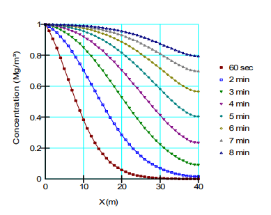
Figure 4. Concentration profiles for Case 1.
Figure 5 shows the concentration distributions for Case 2 that makes use of the source concentration boundary condition. The left boundary has a specified source concentration at the start of the analysis of 1 Mg/m3. Mass is therefore entering the domain at a rate of 𝑞 × 𝐶 at the onset of the analysis; however, mass flux is occurring by both advection (𝑞 × 𝐶) and dispersion (𝑛 × 𝐷 × 𝑑𝐶/𝑑𝑥) immediately inside the domain because of the concentration gradient. As a result, the concentration at the boundary must be less than 1.0 Mg/m3 until the concentration gradient approaches zero, making the advection mass at the boundary equal to the mass flux inside of the domain. The concentration contours become perpendicular to the left boundary as the concentration gradient
approaches zero after about 8 minutes.
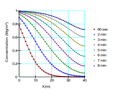
Figure 5. Concentration profiles for Case 2.
Figure 6 compares the concentration distribution for Case 3 to the closed-form solution for a free-exit boundary condition. The CTRAN/W solution compares favourably to the analytical solution. The concentration curves are no long perpendicular to the exit boundary as mass is leaving the domain by both advection and dispersion.
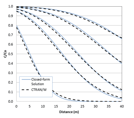
Figure 6. Concentrations with time when the boundary on the right is a Free Mass Exit type compared to the closed-form solution.
Figure 7 presents the results for Case 4 in which the exit boundary was defined using a total mass flux equal to 0 Mg/sec. The concentration at the exit ultimately becomes larger than the source as the mass accumulates at the exit. The application of a total mass flux boundary condition was required to stop mass from leaving the domain by advection. Again, only the divergence of the dispersive mass flux is implicitly zero if a boundary condition has not been applied.
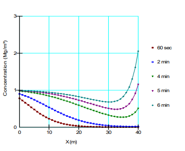
Figure 7. Concentrations with time when a zero mass flux boundary condition is applied to the exit.
Summary and Conclusions
The main objective of this example was to compare results obtained using two options for the source boundary and two options for the exit boundary. The constant concentration boundary condition forces the concentration at the source to remain constant, while the source boundary condition allows the concentration at the source to increase with time until it reaches the specified concentration.
Mass can leave the domain via advection when water is flowing out of the domain, even if the boundary condition is unspecified. This occurs because the natural boundary condition for a solute transfer formulation is zero divergence of the dispersive mass rate. The free exit mass flux boundary condition should be used if dispersion is also expected to remove mass at the exit boundary. The zero mass flux boundary condition is required for scenarios where the water is flowing out of the domain, but the mass cannot leave the domain. This may lead to a higher concentration at the exit boundary than at the source.
The last objective of this example was to compare the numerical solution of the source concentration and free exit mass flux boundary with the closed-form solution of the advection-dispersion equation with a free exit boundary. The results compared well with the closed-form solution, indicating that CTRAN/W implementation is consistent with the theoretical formulations.
References
Frind, E.O., 1988. Solution of the Advection-Dispersion Equation with Free Exit Boundary. Numerical Methods for Partial Differential Equations, Vol. 4, pp. 301-313.