SEG-Y Importer in Oasis montaj

Overview

Video Transcript

[00:00:00.720]
(lighthearted music)

[00:00:11.990]
<v ->Hi everyone.</v>

[00:00:12.823]
My name is Sean Goodman.

[00:00:13.950]
I’m a technical analyst in our UK office.

[00:00:16.060]
And what I’m going to be quickly running through today

[00:00:18.500]
is the new SEG-Y Importer in a ways it’s montage

[00:00:21.350]
and I’ll show you how you can link it

[00:00:22.860]
into building some GM-SYS profile models.

[00:00:26.230]
So the new importer is found in a “3D view” menu

[00:00:30.000]
down at the bottom here.

[00:00:31.010]
So it’s “Import SEG-Y”.

[00:00:33.300]
Now, what we can do is we can select

[00:00:34.870]
between 2D or 3D volumes

[00:00:37.800]
and in time or depth as well.

[00:00:39.900]
So here I have a 3D volume as just a SEG-Y file

[00:00:43.610]
and it’s in time.

[00:00:45.430]
What I can now do once I’ve selected

[00:00:46.910]
my file is look at the text header.

[00:00:49.720]
If you are entirely at the mercy of your seismic processes,

[00:00:53.450]
in terms of how well these are filled out,

[00:00:56.098]
and then you can look at the binary header file

[00:00:59.810]
and the Trace Viewer File.

[00:01:01.770]
And what we can do is we can select the buy order here.

[00:01:04.250]
So big-endian or little-endian, trace data format.

[00:01:08.800]
And we can vary through the current traces to see what they

[00:01:11.340]
look like.

[00:01:15.790]
So I’m going to click next now.

[00:01:19.230]
And again, here we come to the, the key field locations.

[00:01:22.460]
We can define the bites order.

[00:01:24.350]
We can look at the samples per trace interval,

[00:01:26.950]
and first sample at,

[00:01:28.850]
again we can select the trace data format,

[00:01:31.250]
but all of this will be standardly filled out automatically.

[00:01:42.320]
So once we get to the coordinate mapping section,

[00:01:44.630]
we can define the coordinate system here.

[00:01:47.900]
Everything else will be automatically filled out again,

[00:01:50.160]
including the Inline and the Crossline coordinate

[00:01:52.620]
X and Y coordinates.

[00:01:54.570]
So I’m going to fill out the coordinate system here

[00:01:57.540]
based on another grid that I have in this project,

[00:02:02.480]
and that will automatically update

[00:02:04.000]
the projection method and data.

[00:02:09.490]
So here I can select the source of the tie points.

[00:02:12.960]
So that’s either calculated from the trace headers

[00:02:15.910]
or user supplied.

[00:02:17.840]
I can define an output survey file and all of this is

[00:02:21.510]
automatically populated again, based on the input files.

[00:02:30.660]
So here I can actually select to a dummy top and bottom

[00:02:34.290]
traces based on a certain value.

[00:02:37.590]
So I’m going to select zero for this one.

[00:02:40.020]
If we’re bringing in a very large 3D volume,

[00:02:42.330]
then we can subsample the volume so that we don’t bring the

[00:02:45.130]
whole thing in and, and spend a lot of time processing it.

[00:02:51.600]
And the output files here. So we can generate a voxel.

[00:02:55.760]
We can select certain slices to generate

[00:02:58.330]
and we can generate database as well.

[00:03:00.510]
So here I’ve got the Voxel ticked

[00:03:02.730]
and I’m going to generate some slices

[00:03:05.970]
and these are preselected.

[00:03:07.440]
So I’ve got some Inlines.

[00:03:09.250]
I can select some Crosslines

[00:03:11.550]
and some Horizontal Z slices,

[00:03:15.600]
and now I just press, “OK”.

[00:03:16.433]
And that will run and load those in.

[00:03:22.180]
So once that’s loaded in, what that creates is the Voxel

[00:03:25.350]
within the menu here,

[00:03:27.260]
and a series of section grids in the grid menu.

[00:03:30.390]
So “IL”

[00:03:32.111]
“XL”

[00:03:33.020]
and “Z”

[00:03:33.853]
So we’ve got,

[00:03:34.686]
Inlines, Crosslines and Z slices within these grids.

[00:03:38.550]
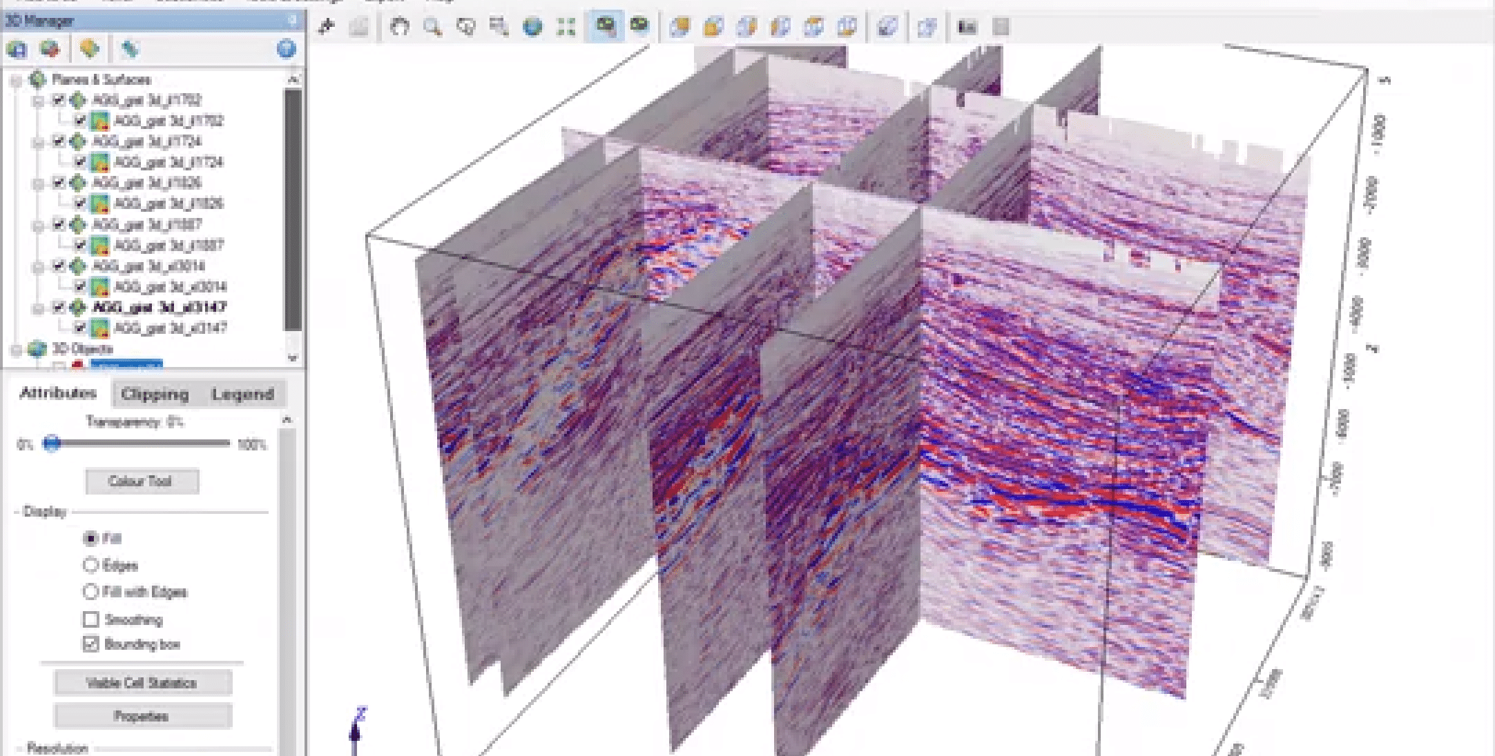
And now what I can do is create a new 3D view so that I can

[00:03:42.380]
have a look at all of these together.

[00:03:53.330]
So I can just drag and drop my 3D Voxel into the 3D view.

[00:04:02.690]
And as you can see the color tool for the Voxel,

[00:04:06.360]
even though it’s seismic is in the

[00:04:07.770]
traditional gravity colors.

[00:04:10.080]
So here, I’m going to select “Color Tool”

[00:04:14.925]
and I’m going to move towards a Seismic Colorbar.

[00:04:21.370]
And then once I’ve done this,

[00:04:22.410]
I’m going to save this as a transform.

[00:04:29.870]
And this means that I’ll be able to apply this to any other

[00:04:32.290]
grids that I add into the 3D view.

[00:04:39.020]
So now I’m going to add in some of those section grids that

[00:04:42.300]
we imported

[00:04:47.090]
and I’ll just go through and select the ones that I want

[00:04:49.510]
from the menu here.

[00:04:54.171]
And what I can go to is my color tool again.

[00:04:57.360]
And I can actually browse for the transform file that I just

[00:05:00.450]
previously created.

[00:05:04.430]
And what this will now do is add that,

[00:05:06.950]
add all of those grids in

[00:05:08.530]
and apply that same color tool to all of the grids at the

[00:05:11.380]
same time,

[00:05:12.213]
without me having to manually go through

[00:05:14.160]
and update each individual one.

[00:05:23.840]
So now we have a seismic sections within the 3D view.

[00:05:29.070]
We can also show our

[00:05:35.830]
voxel

[00:05:37.317]
and what we can do is clip various

[00:05:40.750]
various points.

[00:05:44.740]
So we can clip in the “Z” orientation or from the top.

[00:05:49.570]
We can see how that varies with depth.

[00:05:53.240]
We can clip in the Y orientation and slide through

[00:05:57.250]
and see how the structures vary

[00:05:59.800]
and again in the X orientation.

[00:06:13.930]
So what we can now do,

[00:06:15.060]
if we want to make some GM-SYS Profile Models from those

[00:06:17.530]
section grids, that we’ve just imported,

[00:06:19.330]
we can go to section tools and save those section grids

[00:06:22.820]
to a database.

[00:06:24.930]
Now in this input grid files,

[00:06:26.680]
we can select numerous Inlines and Crosslines and save them

[00:06:30.630]
to a single database here.

[00:06:34.500]
So what this does is for each of those selected lines,

[00:06:38.110]
we now have X, Y and elevation channels defined.

[00:06:43.040]
So this makes it easy for us now to just

[00:06:45.060]
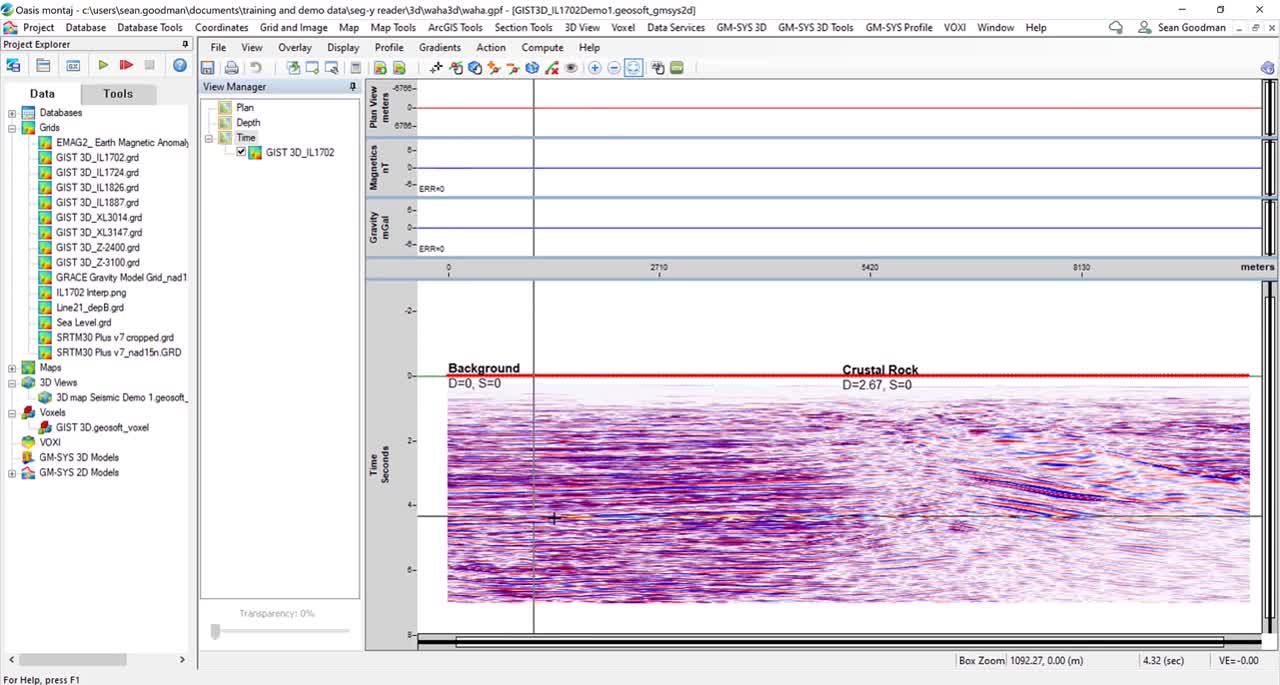
go to GM-SYS profile and create a new time model.

[00:06:55.470]
So we’re going to import from the database line,

[00:06:59.100]
and we’re going to

[00:06:59.933]
we’ve navigated to that, the demo lines one database,

[00:07:04.000]
and we’re going to make a model for Inline 1702.

[00:07:12.350]
So as you’ll now, see, it looks slightly different

[00:07:14.790]
in GM-SYS, this is a result of the 9.8 update.

[00:07:17.810]
So we now have a view manager on the left-hand side.

[00:07:21.730]
What we can actually do is import numerous section grids

[00:07:27.640]
in the depth and time windows. We can also bring,

[00:07:32.510]
we have full format functionality,

[00:07:34.320]
so we can bring things into the plan view window as well.

[00:07:37.640]
So actually what I’m now going to do is add in a new grid.

[00:07:42.160]
One of those section grids for this line,

[00:07:44.920]
this is geo-referenced automatically.

[00:07:47.120]
So I can select that grid file there.

[00:07:50.190]
I can remove the shadow and this,

[00:07:52.620]
this shows me the color that it’s going to use as well.

[00:07:55.290]
And I can select the target pane to be the time section.

[00:07:58.950]
So now that’s immediately brought that in and I can then go

[00:08:02.290]
and digitize any horizons along there and start to build out

[00:08:05.250]
a model as well.

[00:08:06.660]
What I can also do if I’ve got a predetermined image,

[00:08:11.090]
which is geo-referenced within Oasis montage,

[00:08:14.280]
I can now display an image as well.

[00:08:16.930]
So in this example,

[00:08:17.980]
I’ve just drawn some lines over a PNG of Inline 1702,

[00:08:23.410]
and geo-referenced it.

[00:08:24.730]
And now I can bring that into the time section as well,

[00:08:27.700]
and that will overlay that here as well.

[00:08:29.760]
And so I’ve got some interpreted sections on there as well,

[00:08:33.590]
and now I can switch between the two.

[00:08:38.770]
So that’s how you can build out models quite easily

[00:08:42.460]
from the SEG-Y Importer.

[00:08:45.830]
So that’s, that’s all we’re covering off today.

[00:08:47.780]
So, so thanks a lot for watching and good luck.