


Introduction
Many introductory geotechnical engineering textbooks include an example explaining the scenario of water seepage through an embankment. It is, consequently, useful to model this case with SEEP/W, as most users will have an idea of what the solution should look like. The objective of this example is to compare SEEP/W results with a familiar example scenario, as well as to illustrate the analysis of various scenarios by adding multiple analyses and simply changing boundary conditions and material properties.
Numerical Simulation
The model is a 10-m high embankment dam with 2:1 side slopes (Figure 1). Four cases will be analyzed in this example, with an embankment impounding a reservoir that is 8 m deep. The first case will include a single, homogeneous embankment, with seepage occurring along the downstream face. The second case will consist of the same, homogeneous embankment, with an under-toe drain changing the phreatic surface. Initially, the intention is to look at the homogeneous case. The last two scenarios that will be analyzed consist of a clay core within the embankment that has lowered hydraulic conductivities.
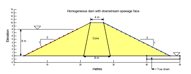
Figure 1. Problem configuration.
The ‘Silt’ sample function included with SEEP/W was used with a saturated hydraulic conductivity (Ksat) of 1×10⁻⁵ m/sec (Figure 2). Since all analyses are conducted using the steady-state conditions, the volumetric water content curves are not required, as no change in storage within the embankment will occur. This curve, however, was included for all analyses to help estimate the hydraulic conductivity function, by using the ‘Silt’ sample material with a saturated water content of 0.45 (Figure 3).
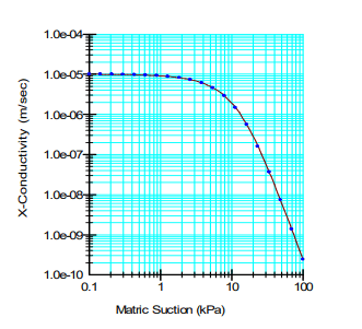
Figure 2. Hydraulic conductivity function of the ‘Silt’ sample material.
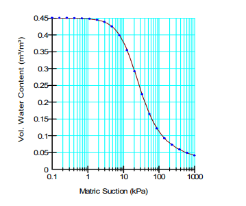
Figure 3. Volumetric water content function of the ‘Silt’ sample material.
The effect of the reservoir can be specified with a total head h boundary equal to 8 m. This creates a pressure head (hp) of 0 m at the elevation of 8 m (h – hp = 8 – 8 = 0) and of 8 m at an elevation of zero (8 -0 = 8). The total head h at the point representing the downstream toe is set to 0 m.
It is anticipated that there will be a seepage face on the downstream slope. The size, however, is not known and, therefore, must be determined by SEEP/W. This is done by specifying a potential seepage face boundary condition by choosing a Water Rate (Q) boundary condition of 0 m3/sec and toggling on the Potential Seepage Face Review option as shown in Figure 4.
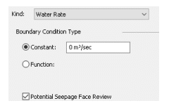
Figure 4. Specified conditions for a potential seepage face boundary condition.
In the second analysis, the toe under-drain is considered to be so coarse relative to the embankment that no energy will be lost in the drain itself. This means that tail water elevation will be at the top of the drain under the embankment (Figure 5). All material properties and the reservoir total head boundary condition are kept the same.
The effect of the drain can be modeled simply by specifying a total head equal to zero along the top of the drain where the embankment and drain are in contact. This is sometimes un-appealing from a presentation point of view. So an alternative is to give the toe drain a material but then specify the total head boundary on the entire region representing the drain as in Figure 5. Note, there is no potential seepage face review on the downstream slope since all the seepage will enter the drain.
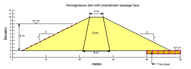
Figure 5. Dam configuration with a toe under-drain.
In the third analysis, a clay core has been added to the analysis by adding a material with a new hydraulic conductivity function that has a lower Ksat. This function is then assigned to the core region (Figure 6). For this example, the same volumetric water content function is used for the core as for the above homogenous cases, and the hydraulic conductivity is estimated with the Ksat is lowered by a factor of 10. A fourth analysis was also included, with the Ksat of the core lowered even more by a factor of 100. A comparison of the three hydraulic conductivity functions can be seen in Figure 7.
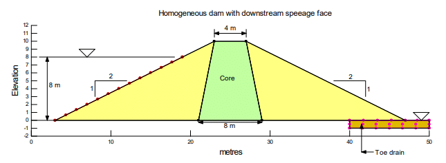
Figure 6. Dam configuration with a clay core.
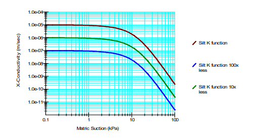
Figure 7. Comparison of the core material hydraulic conductivity functions to the embankment.
Results and Discussion
Figure 8 presents the resulting steady-state, homogenous condition without a toe under-drain. The dashed line is a line where the pore-water pressure is zero. The contours shown are total head contours or equipotential lines (the energy potential along these lines is a constant). As expected, a seepage face is present on the downstream slope.
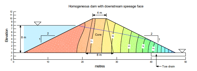
Figure 8. Equipotential lines for the homogeneous case.
Figure 9 shows the flow vectors, which provide a sense of direction and rate of flow. The longest vectors indicate the areas of highest flow rate. Where the flow is extremely low, such as in the crest and upstream toe areas, the vectors become so small that they are not visible. Notice the vectors above the zero-pressure line, which represent the flow in the capillary zone. The vectors also reveal the flow out of the domain occurring along the seepage face.
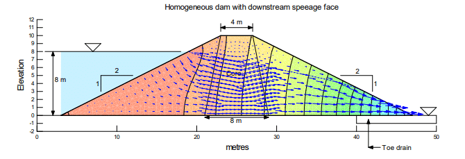
Figure 9. Flow vectors for the homogeneous case.
Figure 10 shows three flow paths that were added. Note, these are NOT flow channels as in a flow net, but indicate paths that a droplet of water will follow through the embankment. Even though they do not represent flow channels, they nonetheless make it possible to provide the appearance of a flow net – at least in part.
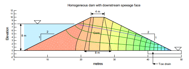
Figure 10. Flow paths for the homogeneous case.
As in a flow net, the flow paths cross the equipotential lines at right-angles. The flow path above the zero-pressure line represents the flow in the tension-saturated capillary zone.
The quantity of seepage through the dam can be determined with the Draw Graph command. Selecting the options as in Figure 11 for the downstream face gives a graph with one data point. The total seepage rate is -1.222e-5 m3/sec. The negative sign indicates flow is occurring out of the domain.
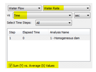
Figure 11. Settings for a seepage quantity graph.
Figure 12 shows the flow regime with the under-drain added to the homogeneous case. As expected, the drain prevents the development of a seepage face on the downstream side of the dam. All of the seepage, instead, goes into the drain.
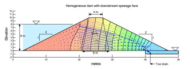
Figure 12. Flow regime with a toe under-drain.
Notice that a significant amount of seepage flows into the drain through the capillary zone where the pore-water pressure is negative. Figure 13 shows the amount of flow into the drain at each of the nodes along the top of the drain. The total into the drain is 1.53e-5 m3/sec.
The graph in Figure 13 is created using a subdomain and then selecting the geometry line along the top of the drain as the location (Figure 14). In this case, the subdomain can be selected by simply clicking on the geometry line between the embankment and the drain, causing all connecting elements to be chosen for the subdomain. It is important to note that most of the seepage into the drain arrives through a zone where the pore-water pressure is negative.
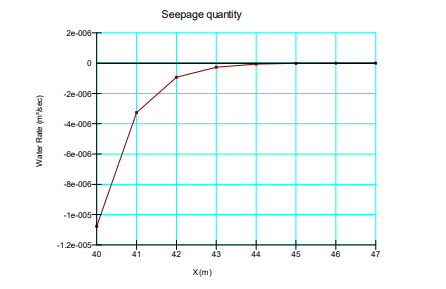
Figure 13. Flow into the drain at each node along the top of the drain.
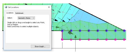
Figure 14. Choosing geometry item for subdomain.
Figure 15 shows the flow regime for the third case, where the Ksat of the core is 10x less than Ksat of the shell material. The large drop in the zero-pressure line within the core indicates that much of the potential energy is dissipated in the core.
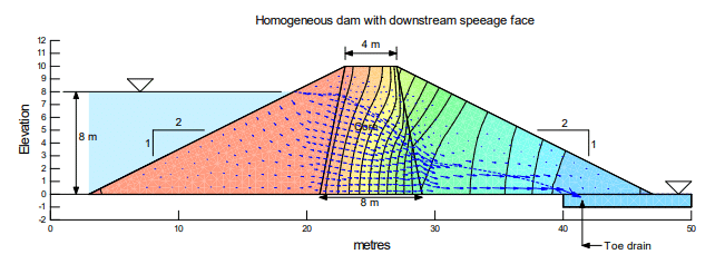
Figure 15. Flow regime with core Ksat reduced 10x.
We can look at the amount of seepage through the core using the same approach as above for seepage into the drain. Here, it is convenient to select the core region as the subdomain and then select either the upstream or downstream line as the location. On the up-stream line, the flow into the core is +4.43e-6 m3/sec. On the downstream line, the flow out of the core is -4.43e-6 m3/sec. The magnitude is the same as it must be under steady-state conditions. The positive (+) sign means that flow is into the subdomain and the negative (-) sign means flow is out of the subdomain.
The resulting flow regime for the last analysis, where the core Ksat is 100x less than Ksat of the shell material, is depicted in Figure 16. Now, almost all of the 8 m potential head from the reservoir is dissipated within the core. The total seepage through the core is now 5.39e-7 m3/sec.
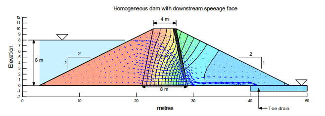
Figure 16. Flow regime with core Ksat reduced 100x.
Once again, it is important to note that there is flow in the zone where the pore-water pressure is negative. It is interesting to look at a flow path that starts at the reservoir surface (Figure 17). A droplet of water would enter the embankment in a saturated zone (pore-water pressure positive) and continue in a saturated zone through much of the core. But then it would enter an unsaturated zone on the way to the drain.
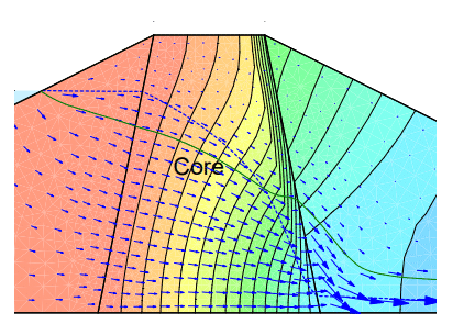
Figure 17. Flow in the unsaturated zone where the pore-water pressure is negative.
Summary and Conclusions
This example provides an illustration of a simple water transfer scenario with multiple analyses considering different material properties and boundary conditions of an embankment. The example demonstrates the changes in the phreatic surface, flow paths and seepage rates when a toe under-drain is added, as well as when a clay material with decreasing hydraulic conductivity is added to the core. The use of subdomains is also introduced to illustrate seepage rates that occur within the domain past geometry items or nodes.