


The Ground-based towed TEM extension is a powerful tool for processing and inverting data. With support for LCI and SCI inversion, it’s integrated with the GIS interface and designed to handle big datasets. It applies efficient processing filters for GPS and voltage data to obtain optimal data quality. Its user-friendly interface enables precise, fine-tuning data processing. To obtain the best possible resistivity model, the inversion also models transmitter waveform and loop shape, front gate filter, and low pass filters, with the option to set these as hard parameters or soft constraints. Modelling and presentation to the customer are done with the well-known functions of the Workbench, making it easy to integrate with boreholes, create reports, and more.
Key features
- Efficient and easy-to-use data processing tools and filters
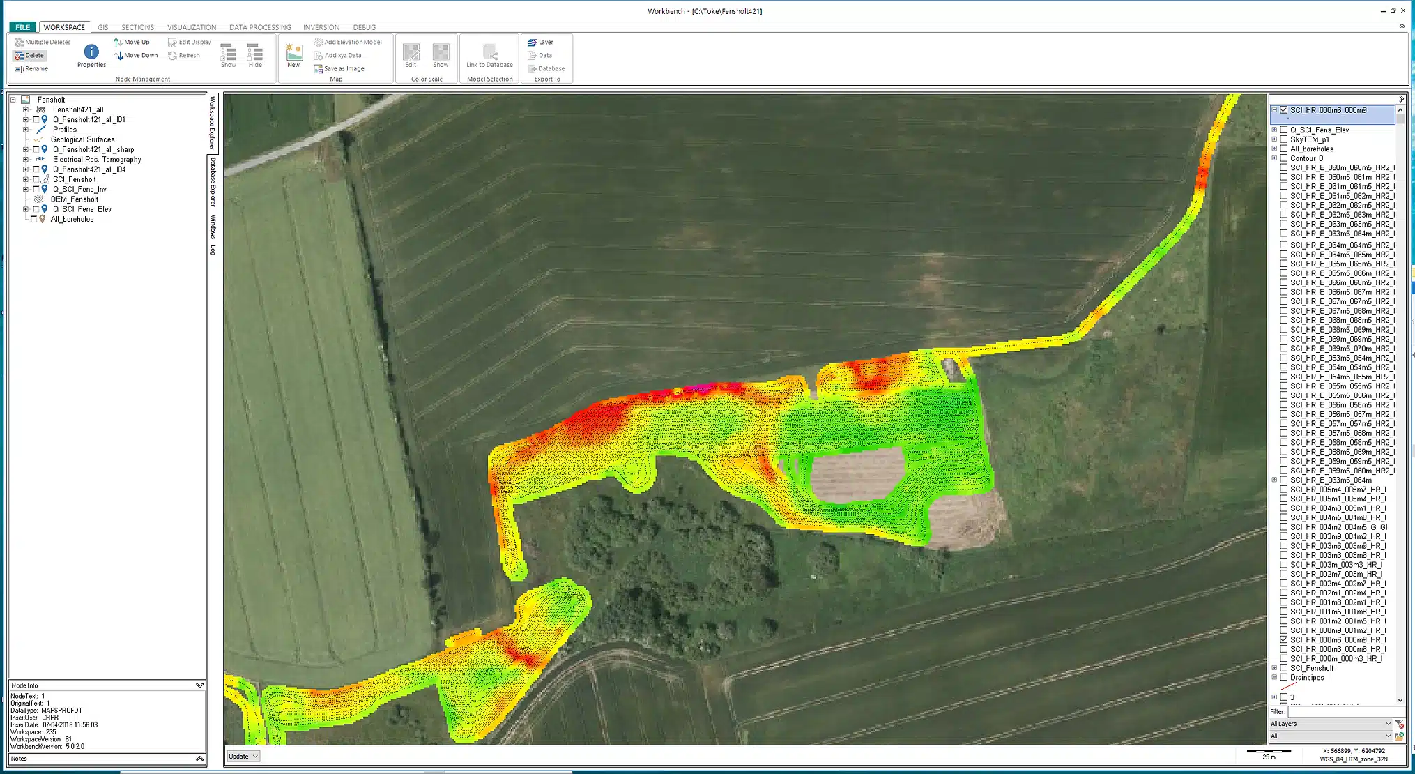
- Integrated GIS user interface with borehole display
- Thematic map and cross-section model visualisation
- Quality Control (QC) visualisation tool for both data and inversion
- Laterally or Spatial constrained inversion using the AarhusInv algorithm
- Parallel computing compatibility for efficient inversion distribution across computers
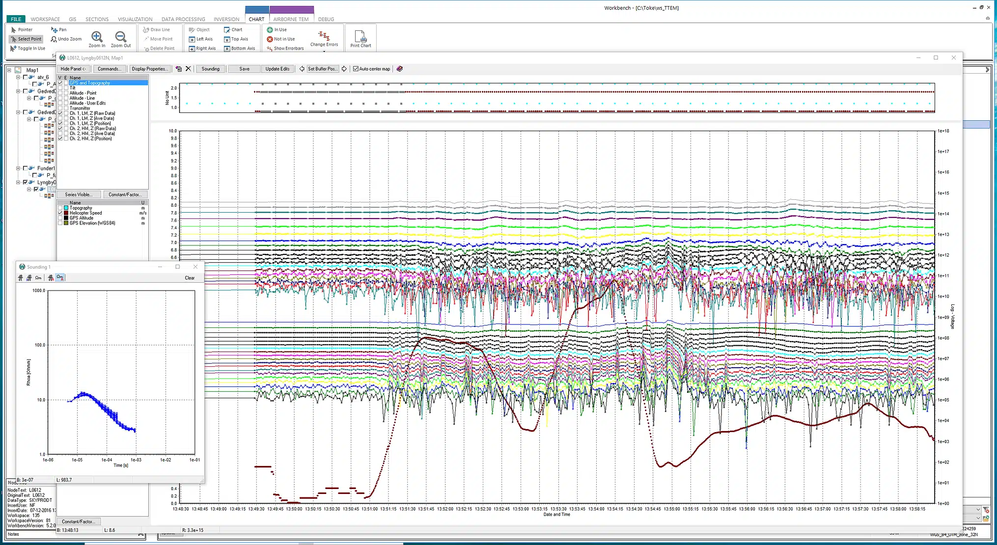
Processing
Tailored to handle large datasets, this extension organises data in a comprehensive database structure with detailed information on the ground-based system. It simplifies the EM data processing and inversion process, making it accessible even for non-experts. The database not only archives raw and processed data but also records all processing steps and settings for documentation. The processing is performed with user-adjustable automatic data filtering and stacking. You can inspect the automatic processing at different levels and add user corrections through the interface. The processing features include:
GPS
-
Path tracking to close minor gaps in the GPS records and for filtering outliers
-
Lag correction to move the transmitter-receiver coil configuration to the optimal focus point
-
Support for differential GPS and digital elevation model from the GPS or from external grid
Voltage data
-
Filtering of distorted data due to EM coupling to power lines and cables
-
Adjustable trapezoid-shaped stacking for optimizing and balancing the signal-to-noise ratio and lateral resolution.
-
Data uncertainties estimated from the stacked data
-
Manual inspections and corrections to the single data point level
Inversion
Data can be imported into Workbench with key system parameters grouped in a separate data file. After import, you have full access to the comprehensive inversion modules as well as the processing extension.
To have full control of the data processing phase we advise importing raw data for optimal processing control in Workbench, though pre-processed data can also be imported for inversion.
Constraints
Inversion of TEM data in Workbench is performed with the AarhusInv code. Locally we use a 1D model. The models are laterally and spatially constrained forming pseudo 2D and 3D model spaces. The inversion code has been customized to handle data from very big TEM surveys and supports multi-CPU cores with very high parallel efficiency. Besides providing the resistivity models, the inversion code also calculates a depth of investigation (DOI) and a data residual for each resistivity model.
-
LCI-setup: Lateral constraints along flight lines forming at 2D model space.
-
SCI-setup: Lateral constraints along and across the flight lines for a 3D-constrained model space. A full survey can be inverted as one single SCI setup.
The lateral constraints can be applied in depths or elevations, giving you more control over the modelling process.
Model types
Workbench offers three main types of model discretization/regularization schemes. These schemes affect the smoothness or sharpness of the model results. Users can adjust the strength of the constraints and the regularization schemes. The model types are:
-
Smooth: The resistivity model is discretised using several layers (~10-20) with fixed layer boundaries. The regularization penalizes vertical changes in resistivity, resulting in a vertical smooth resistivity model.
-
Sharp: The resistivity model is discretised using several layers (~10-20) with fixed layer boundaries. The regularization penalizes the number of vertical resistivity transitions of a certain size, resulting in resistivity models with relatively sharp vertical resistivity transitions. The sharp regularization scheme can also be applied to the lateral constraints.
-
Layer: The resistivity model is characterized by a few layers (~4-5). Both layer thickness and resistivity are model parameters. No vertical regularization is applied which results in distinctly layered resistivity models with a fixed number of layers. A built-in routine estimates the number of layers needed to fit the dataset based on smooth model inversion results.
Prior constraints
Workbench also supports prior constraints on any model parameter. The prior constraints can be initialized from grids and directly from the GIS map, or specified at borehole locations with decreasing strength moving away from the borehole locations.
Accurate system modelling
To obtain high-quality inversion results it is important to model the EM system in great detail. The following parameters are included:
-
The shape of the transmitter loop
-
Transmitter waveform
-
System low-pass filters
-
Front gate filter
-
Width of the individual time gates