Processing Conditional Simulations in Leapfrog Edge with GeoEstima

Post-processing of the block model will quantify the uncertainty in the resources for the mineralised domains, enabling informed decision making. In this webinar, an overview of the procedure to generate the conditional simulations will also be covered.

GeoEstima is an economic geological consultancy company in Santiago Chile, founded in May 2013 by Orlando Rojas.

About the speaker: Orlando Rojas is a Geologist (University of Chile) and a geostatistician (Ecole des Mines de Paris). He has 27 years of experience in mining and geology, with a specialisation in the evaluation of Mineral Resources, Geometallurgy and Geostatistics.

Video Transcript

[00:00:00.546](upbeat music)

[00:00:11.938]<v Host>Hello and welcome. (sound echoing)</v>

[00:00:14.609]Here at Seequent, we are always looking to improve

[00:00:16.960]our solutions to enable our users

[00:00:19.030]to solve increasingly complex problems, manage risk,

[00:00:22.040]and gain valuable insights from their data.

[00:00:25.100]So I’m excited to introduce Orlando Rojas,

[00:00:27.720]as our presenter in this webinar,

[00:00:29.240]in Processing Conditional Simulations in Leapfrog Geo.

[00:00:33.040]Orlando is a respected Geologist

[00:00:35.280]and Geostatistician with hands-on experience,

[00:00:38.151]beginning in 1993, as an exploration Geologist,

[00:00:41.880]working on various projects through to mining production.

[00:00:45.290]Which has led to him to specialize in resource estimation.

[00:00:51.460]He has rounded off his education with a diploma

[00:00:53.720]in Geostatistics from the hallowed Paris School of Mines,

[00:00:57.010]and has even started his own successful consulting company,

[00:01:00.990]GeoEstima, which he operates out of Santiago Chile.

[00:01:05.120]He has published papers on the use of Conditional Simulation

[00:01:08.110]and he spoke at the Seequent Lyceum in September

[00:01:10.700]on the past, present and future of Geostatistics,

[00:01:13.710]which is now on our, open our webinar, sorry,

[00:01:15.830]up on our website if you’re interested in checking that out.

[00:01:19.580]This leads us onto today’s topic of Conditional Simulation.

[00:01:23.560]Have you wondered how to integrate them into your estimates

[00:01:26.040]in leapfrog Geo but not sure how or where to start?

[00:01:29.250]Orlando is going to demystify this process,

[00:01:31.610]giving you practical tips on how to do this

[00:01:34.230]when you get back into the office later.

[00:01:36.950]Orlando, it’s over to you.

[00:01:40.030]<v Orlando>Well, good afternoon.</v>

[00:01:41.950]Good morning everywhere, thanks Gary,

[00:01:44.500]for the introduction, invitation,

[00:01:47.930]we are glad by the opportunity to show our work

[00:01:51.960]to professional on this part of the world,

[00:01:55.120]many thanks to Seequent, for the invitation and trust.

[00:01:59.320]I hope that the contents of this webinar

[00:02:02.690]are of interest to you.

[00:02:06.656]GeoEstima is an independent privately owned

[00:02:09.430]consultant company serving the global mineral industry.

[00:02:13.660]And the company has been in the market since 2013,

[00:02:18.500]but our director, staff and associate have world experience

[00:02:23.190]in mining mineral resource, evaluation, geometallurgy,

[00:02:28.176]and exploration.

[00:02:30.720]We are based in Santiago, but we have a… (clears throat)

[00:02:35.030]A lot of client around the world

[00:02:37.620]mainly in South America, but also in Spain, Africa and USA.

[00:02:46.110]Where key commodity focus include copper,

[00:02:48.840]molybdenum, copper gold, gold silver, zinc, lead,

[00:02:52.960]lithium, hard rock and iron, (clears Throat)

[00:02:58.203]The agenda for today is the presentation name,

[00:03:02.290]Processing Condition Simulation in EDGE

[00:03:05.870]and update at the end,

[00:03:07.780]we are going to answer a couple of questions

[00:03:11.160]for more specific question, please, don’t not hesitate

[00:03:16.540]to send us an email after this webinar.

[00:03:24.130]In this presentation, the topics to be present are,

[00:03:27.490]implicit data and implicit geological modeling.

[00:03:32.050]A very brief overview of conditional simulations,

[00:03:36.380]how to perform conditional simulations based on

[00:03:40.770]an implicit data, our work flow to apply this methodology,

[00:03:47.450]the simulation assessing, and finally,

[00:03:51.500]a discussion of results.

[00:03:56.620]Well, (clears throat) as introduction,

[00:03:59.360]the geological model represent the best approach

[00:04:02.730]of an unknown reality.

[00:04:05.170]These geological models are based on

[00:04:08.180]two fundamental aspects:

[00:04:12.095]The mineral deposit knowledge,

[00:04:15.110]that means the style of mineralization

[00:04:17.550]or type of deposit commodity

[00:04:20.610]or genesis, main control of mineralization,

[00:04:24.550]the structural control, etcetera.

[00:04:26.800]And the quantity and quality of sampling.

[00:04:31.620]What is know as information effect.

[00:04:35.480]All models have uncertainty associated

[00:04:39.440]with and well, we’ll only know the deposit

[00:04:43.600]when this is completely exposed.

[00:04:46.740]Uncertainty refer to epistemic situation involving

[00:04:50.960]imperfect or unknown information.

[00:04:56.202]As Box and Draper said,

[00:04:59.577]“Remember that all models are wrong;

[00:05:03.240]the practical question is how wrong to do

[00:05:06.770]they have to be to not be useful?”

[00:05:12.490]The uncertainty of a mineral resource model is not only

[00:05:17.030]depending on of grade estimation uncertainty,

[00:05:22.511]but also of volume and density.

[00:05:26.370]In fact, the definition of contained metal

[00:05:30.100]is equal to the volume times density times grade.

[00:05:35.700]In this context the volume is determined by

[00:05:39.030]the geological model.

[00:05:41.460]The geological interpretation are key to models

[00:05:45.970]used in the business of mining and such model

[00:05:50.400]are example, examples of scientific models.

[00:05:55.170]The question is how to know the uncertainty associated

[00:05:58.631]to our geological interpretation.

[00:06:02.000]It is well known that from a same data set,

[00:06:06.080]we could create different outputs or scenarios

[00:06:10.700]for a geological interpretation.

[00:06:13.320]For example, Leapfrog Geo,

[00:06:15.680]we can generate different scenarios adjusting the setting.

[00:06:20.860]However,

[00:06:22.970]this has not indicate us which one is the more possible

[00:06:27.440]or probable output.

[00:06:29.780]During mine exploitation reconciliation between long term

[00:06:33.970]and short term models, will give us our realistic measure

[00:06:39.030]about the credibility of the regional model,

[00:06:42.510]but these only apply to the effectively exploited area.

[00:06:51.400]The alternative is modeling the uncertainty based on

[00:06:54.950]the same data set used for modeling and estimates.

[00:07:00.020]Applying conditional simulation.

[00:07:03.292]A geostatistical tool that allows to get a set

[00:07:06.850]of equiprobable scenarios and a measure with probabilities

[00:07:12.045]of the difference in between them.

[00:07:16.820]Okay.

[00:07:19.130]The main objective of this presentation is to show

[00:07:22.510]a case study where conditional simulation

[00:07:25.260]are applied to evaluate different scenarios

[00:07:27.757]and the uncertainty of the geological

[00:07:31.460]model built from an implicit data Leapfrog Geo.

[00:07:35.580]Also we will talk about:

[00:07:38.940]The fundaments behind implicit geological modeling

[00:07:42.440]in Leapfrog Geo, alternatives or path

[00:07:45.890]to stimulate geological variables,

[00:07:48.820]The use of the model’s implicit data based to assess

[00:07:53.370]the models uncertainty with conditional simulations,

[00:07:57.820]discuss the results and show some applications.

[00:08:05.130]The scoping of this case studies.

[00:08:09.370]Build a geological model in Leapfrog Geo.

[00:08:12.930]Extract implicit data related to the

[00:08:16.050]geological surface or solid that we want to assess.

[00:08:21.170]Perform conditional simulations based on this

[00:08:24.110]implicit dataset in another platform for now.

[00:08:28.850]Obtain several scenarios of the geological surface

[00:08:32.010]or solid under study.

[00:08:35.540]All of them with equal probability.

[00:08:39.450]Perform post processing on the simulation results

[00:08:42.970]and make the assessment of the scenarios in EDGE

[00:08:47.430]The scenarios are evaluated later in terms of tonnage,

[00:08:52.140]grade and metal content.

[00:08:58.700]Implicit data is a way to convert a discrete

[00:09:03.860]or categorical geological variable to a continuous variable.

[00:09:09.440]Predict.

[00:09:11.180]A Geological contact (clears throat) between two units,

[00:09:18.760]is express as distance, uptown or down the hall

[00:09:25.440]from the point where the contact is located.

[00:09:29.390]At this point, the zero variable is assigned,

[00:09:32.560]then this distance inward, the unit are measured

[00:09:36.740]as positive.

[00:09:39.461]Otherwise the distance from the zero, I have all the words,

[00:09:45.840]the unit and measure as negative values.

[00:09:54.570]Well, if we can interpolate implicit data,

[00:09:59.880]we can also simulate it.

[00:10:03.110]The geostatistical simulations were date from 70s.

[00:10:06.520]The purpose of simulation is to reflect

[00:10:10.400]the structural characteristic of the revealed reality.

[00:10:16.450]For problems dealing with the fluctuation

[00:10:18.820]of all characteristics simulation is required.

[00:10:24.648]Categorical valuables, the algorithm for simulation

[00:10:28.850]are Sequential indicator stimulation, Truncated Gaussian,

[00:10:34.760]Truncated pluri-Gaussian simulation,

[00:10:37.950]Hierarchical Approach

[00:10:39.450]to Truncated pluri- Gaussian simulation.

[00:10:43.087]And for continuous variables, Sequential Gaussian simulation

[00:10:47.050]and Turning Bands.

[00:10:52.210]The simulation allows us to generate N trial of

[00:10:56.020]the equal probability of one domain based on same dataset.

[00:11:01.710]Recording the difference between each simulation

[00:11:04.890]we could obtain an assessment of uncertainty.

[00:11:09.729]A lower data density will imply greater difference

[00:11:14.030]between outputs.

[00:11:15.390]Conditional simulation output will be the same where data

[00:11:19.360]or a sample exist.

[00:11:22.380]The post-processing of the simulation domains allow us

[00:11:26.110]to have an assessment of variability that we could see

[00:11:30.290]through probability maps, quantiles values,

[00:11:33.410]interval of confidence, etcetera.

[00:11:38.030]In our approach as the categorical variable

[00:11:42.033]or geological variable is convert to a continuous variables

[00:11:46.730]implicit data we could apply some algorithm

[00:11:50.240]for continuous variables

[00:11:52.800]as Sequential Gaussian or Turning Bands.

[00:11:57.340]This approach must deal with some non-stationery

[00:12:01.380]issues related to the distance variable.

[00:12:05.450]That in most case are addressed by clipping of the data

[00:12:10.070]around the surface or 3D solid,

[00:12:13.930]and especially applying local searching methodology known as

[00:12:18.760]local geostatistics.

[00:12:21.150]A practical validation of this process is the comparison

[00:12:25.550]in between the e-type value, processors from the entire

[00:12:30.630]of simulated values in front of the solid

[00:12:34.560]or surface created by Leapfrog.

[00:12:40.780]In these slides we present a simplified workflow

[00:12:44.040]to develop such a study.

[00:12:47.210]The first step is to import the database into Leapfrog,

[00:12:51.840]then build a 3D geological model in Leapfrog.

[00:12:57.763]Extract the implicit database

[00:13:00.530]related to the surface or solid that we want to assess.

[00:13:05.740]Export implicit database for this element,

[00:13:08.880]then import the implicit database into another platform

[00:13:13.270]like, yes Leap or (indistinct).

[00:13:17.368]In this platform, carry out the conditional simulation

[00:13:21.890]using a Sequential Gaussian simulation

[00:13:25.710]or Turning Bands and performed post-process

[00:13:29.730]of the simulation.

[00:13:32.800]Once the simulator are done, the outputs are imported

[00:13:37.640]into Leapfrog to carry out the post-process

[00:13:40.620]and build the different scenarios of the model.

[00:13:50.040]The case study..

[00:13:52.160]This case study will respond to a gold deposit

[00:13:55.610]with a tabular and horizontal shape.

[00:14:00.201]The geological model was built using interpolation

[00:14:05.262]on the Lithological Table

[00:14:07.790]then creating assumed face model,

[00:14:10.190]with Leapfrog new inclusion tool.

[00:14:14.670]After finished the 3D solid implicit data used to build

[00:14:19.640]it was damped to CSB file.

[00:14:25.610]Here,

[00:14:27.000]we present, at right,

[00:14:30.010]the 3D geological modeled in front of grade sample

[00:14:34.340]from recalls

[00:14:36.160]and at left, the geological model in front of

[00:14:39.440]the recent dataset.

[00:14:42.230]Right colors shows positive distance values,

[00:14:46.370]and blue color, the negative distance values

[00:14:49.800]of implicit data.

[00:14:54.660]Methodology to perform the conditional simulation.

[00:14:59.450]The procedure begin importing implicit database.

[00:15:03.400]Then on organized cleaning estimation is performed to keep

[00:15:08.700]the (indistinct) to de-cluster the samples.

[00:15:13.360]The transformation of the real values to Gaussian data

[00:15:17.830]was based on anamorphosis modeling Gaussian,

[00:15:21.650]that might (indistinct).

[00:15:23.840]Then experimental variograms on the Gaussian data

[00:15:27.610]were calculate.

[00:15:30.050]Then the variogram were fit to obtain the biochem models.

[00:15:35.200]With this input, the conditional simulation

[00:15:38.290]were performed using Turning Bands algorithm

[00:15:42.250]that damped 100 realization of the random valuable.

[00:15:48.059]Validation of simulated value were dumped.

[00:15:52.290]Finally, the simulation outputs where post-processes

[00:15:56.250]to obtain the average of the simulation type

[00:16:00.700]on the probability for each block to be inside

[00:16:04.160]or out outside the, the geological boundary,

[00:16:08.240]which one is compute over the entire simulated values,

[00:16:12.590]considering all this simulated distance greater answer.

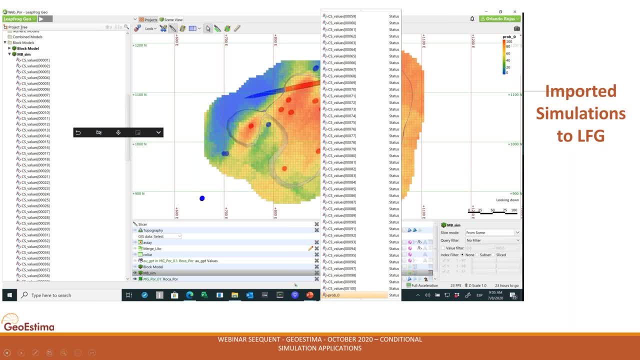
[00:16:21.853]In this is slide, we have an example of the simulate model

[00:16:27.580]already imported to Leapfrog art.

[00:16:31.352]As Shown, the 100 simulation

[00:16:35.565]and the probability of variables in the block model.

[00:16:43.040]This is the cross section where it showing

[00:16:46.910]the implicit data

[00:16:48.260]and the original geological 3D solid build from this data

[00:16:53.970]in front to simulations or realization.

[00:16:58.510]This is the simulation number 10 to 100

[00:17:04.550]A Simulation 20, 30,

[00:17:10.220]40,

[00:17:11.990]50,

[00:17:13.200]60,

[00:17:15.500]70,

[00:17:16.442]80,

[00:17:17.775]90

[00:17:19.357]and 100.

[00:17:23.180]In this slide, we have the probability that shows values

[00:17:27.710]between zero to 100.

[00:17:32.771]Regarding the probabilistic model.

[00:17:34.660]This is built based on the 100 simulated distance

[00:17:39.290]to the contact at each block.

[00:17:42.530]If a particular simulated distance is greater

[00:17:46.230]or equal to zero means at this realization the block,

[00:17:50.910]is inside the geological unit else it is outside.

[00:17:57.000]If we define an indicator, C,

[00:18:00.010]which is one if the distance is greater or equal than zero

[00:18:06.270]else, it is zero.

[00:18:08.900]Therefore the probability will be the sum of C

[00:18:13.680]divided by the number of (indistinct), in this case 100.

[00:18:20.608](clears Throat)

[00:18:21.780]Here, we have an example of the probability modeled

[00:18:26.530]or probability map in a plan view.

[00:18:31.980]The same example in another plan view

[00:18:35.230]here, the probability mold is in front of the dataset.

[00:18:42.600]In this example we have a cross section.

[00:18:48.175]And here are a probability modeled as isometric view.

[00:18:56.412]As, we have the probability we would compute

[00:19:00.150]inside the 3D solid, the range of probability values.

[00:19:04.890]In our case, we could define probability interpass

[00:19:09.434]of 10 by 10,

[00:19:11.190]then use it to assets the uncertainty related to the solid.

[00:19:17.370]In the figure shown here, we can conclude

[00:19:21.670]that a minor (indistinct), less than 10% of blocks

[00:19:26.310]had a probability less than 50%.

[00:19:31.057]And 62% of the blocks have more than 80% of probability

[00:19:36.220]to belong to this geological unit.

[00:19:40.110]Therefore,

[00:19:41.830]this start (indistinct) gives us a quantity assessment

[00:19:46.420]of the uncertainty of this geological interpretation.

[00:19:50.910]Also, it is possible to find some blocks

[00:19:54.620]with greater probability that are outside the solid.

[00:20:01.210]Then we could include these blocks with a new interpretation

[00:20:11.339]Applications.

[00:20:12.422](clears throat)

[00:20:13.530]If we estimate grade inside the domain,

[00:20:17.940]we will obtain a mineral resource evaluation of the orebody.

[00:20:22.790]Then we can subdivide and classify

[00:20:26.720]this evaluation according range of probability

[00:20:31.090]or degree of uncertainty.

[00:20:33.980]Other option is editing the solid with some polylines

[00:20:38.590]to include those nodes or blocks with more probability

[00:20:43.940]or visa versa eliminate those with less probability.

[00:20:48.610]By last, we could complement this uncertainty study

[00:20:53.230]performing the grades conditional simulating and, or

[00:20:57.070]the density.

[00:20:59.560]The complete analysis we be express as

[00:21:03.920]metal contained is equals to

[00:21:08.090]volume plus minus a delta times density

[00:21:12.940]plus minus a delta times grade plus minus delta.

[00:21:21.990]The last that calculation could be done using Script.NET,

[00:21:25.920]as we show in this slide.

[00:21:30.960]Also after class range calculation,

[00:21:35.270]we could report the mineral of resource by class.

[00:21:43.580]Conclusion. (clears throat)

[00:21:45.740]From an implicit geological model in Leapfrog Geo we could,

[00:21:50.770]we could obtain implicit data export it

[00:21:53.879]and apply conditional simulation technique

[00:21:57.370]on the same database which the geological model’s solid

[00:22:01.960]was made.

[00:22:04.440]As the implicit data is a continuous variable,

[00:22:07.680]we could deal the conditional simulation using algorithm

[00:22:12.810]for continuous variable as Sequential Gaussian

[00:22:16.860]and Turning Bands.

[00:22:19.300]The simulation outputs can be post-processed to obtain

[00:22:23.320]the average of the simulation, named e-type

[00:22:27.940]and the probability for each block to be inside

[00:22:31.150]or outside the geological boundary.

[00:22:34.430]Which one is computed over the entire simulated values

[00:22:38.630]considering all the simulated distance (indistinct).

[00:22:44.820]With this information we could subdivide and classify

[00:22:48.650]this evaluation according ranges of probability

[00:22:53.340]or degree of uncertainty.

[00:22:56.790]Also, this information gives us measurable options

[00:23:01.730]to adjust the original model,

[00:23:04.900]as we can make edits if we want

[00:23:08.660]different grades or uncertainty in our model.

[00:23:17.780]Recommendations.

[00:23:20.660]Apply this technique as it is a good alternative

[00:23:25.130]to simulate surfaces or solids of a geological model

[00:23:29.950]and can be related to an implicit model in Leapfrog Geo.

[00:23:35.080]Assessing the uncertainty of the geological model

[00:23:37.760]is recommended task when we would like to have a good

[00:23:42.690]understanding of the risk and opportunities related

[00:23:46.340]to the geological interpretation.

[00:23:49.520]This type of study is used to support

[00:23:53.010]drilling density optimization

[00:23:56.193]and support Mineral Resources classification criteria.

[00:24:01.242]It is possible to use a different type of studies

[00:24:05.410]as exploration, mineral resource evaluation

[00:24:09.340]or mine operations.

[00:24:14.630]This technique has been successfully applied for

[00:24:18.640]very complex geological model, for example,

[00:24:21.810]Skarn-type deposit and with huge database of training.

[00:24:29.096](clears throat)

[00:24:30.310]Here we have an output of…

[00:24:33.600]For a Skarn or body,

[00:24:37.290]and we could see the high similarity between

[00:24:40.410]probabilistic model and implicit model.

[00:24:46.170]Thank you.

[00:24:50.630]<v Host>Thank you, Orlando that was a great talk on,</v>

[00:24:54.570]on conditioner simulation and

[00:24:58.490]definitely thought provoking when it comes to

[00:25:01.580]sort of assessing the uncertainty on our geological models,

[00:25:05.700]which are form the basis of the input

[00:25:07.470]to our resource estimates.

[00:25:09.280]So thank you very much.

[00:25:12.160]So I do have a couple of questions here, I’d like to ask,

[00:25:15.780]so you have mentioned it, but how,

[00:25:19.530]how would the implicit dataset be obtained?

[00:25:24.260]Can you elaborate on that?

[00:25:27.530]<v Orlando>Well, in leapfrog Geo</v>

[00:25:30.040]is based on the implicit dataset

[00:25:35.460]that you could take from the…

[00:25:41.902]The model directly each,

[00:25:44.010]each sort of face or solid Leapfrog

[00:25:46.650]is related to implicit data set.

[00:25:50.290]So do take it very easy from the…

[00:25:55.627]The geological model directly just click into your

[00:26:00.970]right bottom of the mouse.

[00:26:06.170]<v Host>Yeah. Okay, lovely.</v>

[00:26:08.080]Thank you, and…

[00:26:11.030]You also, like in your conclusions,

[00:26:13.410]there were recommendations, you mentioned

[00:26:16.600]using it for resource classification.

[00:26:18.680]How would you go about applying conditional simulation

[00:26:22.550]to resource classification, which is another kind of,

[00:26:27.350]uncertain sort of part of the resource estimation process?

[00:26:33.360]<v Orlando>Well, the, to apply to resource,</v>

[00:26:37.280]near resource classification,

[00:26:41.410]you could relate, you could create relationships

[00:26:44.730]between the variability with different samples, density,

[00:26:50.640]or in some different, three whole spacing.

[00:26:55.633]And

[00:26:57.873]also you need to relate this uncertainty

[00:27:02.090]related to the sample density with different unit of,

[00:27:09.120]mining units for instance, period, unit for instance

[00:27:12.610]one year, or one month.

[00:27:17.570]So if we condition our simulation you could

[00:27:22.153]help and make sure inside this period for some one year

[00:27:28.780]you could check the variability and you could check,

[00:27:32.040]which is your sampling density

[00:27:36.100]inside this area and so

[00:27:39.920]try to get with that way,

[00:27:42.940]the more or less

[00:27:46.560]variability related to the sampling density.

[00:27:50.680]<v Host>Some things to try out there, thank you so much.</v>

[00:27:53.780]Okay, thank you everyone.

[00:27:55.040]Thanks for attending and thank you, Orlando.

[00:27:56.880]Thank you.

[00:27:58.630]<v Orlando>Thanks, bye.</v>

[00:28:00.572]<v Host>Bye.</v>