


Introduction
The preservation of the permafrost is often imperative to protect such structures as roads, railways, and runway embankments. Man-made structures generally alter the surface energy balance in a manner that causes an overall warming trend. Goering (2000) investigated passive cooling within an embankment constructed of unconventional and highly porous materials as means of preserving permafrost. Unstable density stratifications within the porous embankment led to the development of convective cells during the cold winter months. The convective cells enhanced energy transfer out of the earth structure, resulting in a deeper penetration of cold air within the embankment, which in-turn promoted preservation of the foundation permafrost layer. The objective of this example is to simulate similar convective cell behavior that was seen by Goering (2000) using AIR/W and TEMP/W.
Background
Goering (2000) used a finite element program to numerically simulate the heat and air transfer that occurred in a full-scale field test (Goering and Kumar, 1996 and Goering, 1998). Goering (2000) focused on the air pressure boundary condition for the side-slope of the embankment and gave consideration to: (a) an open boundary which allowed for infiltration of ambient air; and b) a closed boundary which allowed for internal convection and no interaction with the atmosphere. The closed boundary represents, for example, high moisture content topsoil covering the porous embankment or snow cover during the winter months.
Numerical Simulation
Figure 1 presents the finite element domain used to represent the porous roadway embankment and underlying foundational soil. The symmetrical nature of the problem allowed only half of the domain to be simulated. The embankment roadway is 6 m wide, 2.5 m in height, and has 2:1 side-slopes. The mesh density was increased within the embankment and below the interface with the foundation, but decreased (i.e. element size increased) along the outside edges of the lowest region.
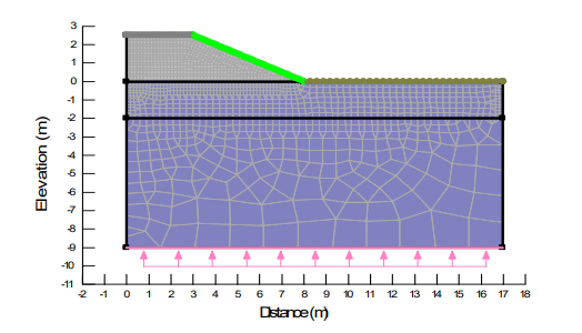
Figure 1. Finite element domain.
The Project File comprises three analyses (Figure 2). The initial conditions are completed by simulating steady-state air and heat transfer analysis on the same domain. The free convection option has been toggled on within the Physics tab of the Project Settings (Figure 3). As a result, the initial temperature distribution affects the air density, which in-turn affects the steady-state initial pore-air pressure distribution.
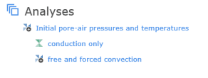
Figure 2. Analyses Tree for the Project.
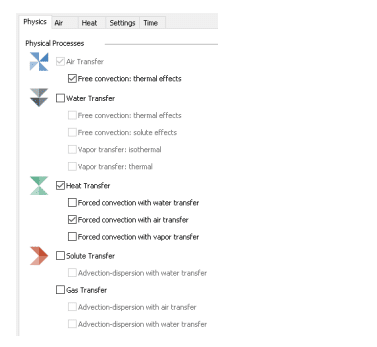
Figure 3. Physics tab settings for the AIR/W and TEMP/W analyses.
The first transient analysis has been created to simulate the effects of conduction only on the heat transfer within the slope, and only considers the heat transfer conduction processes on the domain. The second transient analysis has both air and heat transfer processes and has toggled on the option for forced convection with air transfer, which means that heat energy is moving within the domain because of both conduction and advective processes. The multi-physics formulation uses the air fluxes to compute and assemble the advective heat (energy) transfer terms into the global finite element equations. Notice that no consideration is being given to the existence of water within the domain. Water transfer, and possibly forced convection with the water flow, could also be simulated by adjusting the settings on the Physics tab of the Project Settings.
Ignoring the presence of water within domain allows both the foundation and embankment soils to be represented by the single phase air material model. The foundation soil is silt with high moisture content; therefore, a negligible air hydraulic conductivity of 0.001 m/day was assumed. A non-zero value for air conductivity is required even if the soil is saturated so that the finite element equations can be solved. The arbitrary value should not be unnecessarily small to prevent numerical ill-conditioning of the global finite element matrices.
Goering (2000) reports an intrinsic permeability k for the granular embankment material of 6.3×10 – 7 m2. The intrinsic permeability of a fluid is related to the hydraulic conductivity (𝐾) by:
𝑘 =𝐾𝜇 /𝛾
(Equation 1)
where 𝜇 is the dynamic viscosity and 𝛾 is the unit weight. Assuming that 𝜇 = 1.78 × 10 ‒ 5 𝑘𝑔 (𝑚 ‒ 𝑠) and 𝛾 = 11.81 𝑁 𝑚 results in an air hydraulic conductivity of approximately 36,000 m/day. The air fluxes are used to compute and assemble the advective heat (energy) transfer terms into the global finite element equations. Extremely large air fluxes, created by the use of extraordinarily high air conductivity, can create ill-conditioned global finite element matrices, resulting in premature termination of the solvers. An analysis of this type should generally be developed by incrementally increasing the air conductivity so that numerical stability can be judged by comparison of results. Such an approach is particularly important when both water and air transfer is being simulated because mathematically coupled formulations are prone to numerical instability because of extraordinary contrasts in the hydraulic properties.
Goering (2000) did not indicate the value of dynamic viscosity. The only value supplied in the paper was the intrinsic permeability. As such, the exact value of the air conductivity is unknown. The analysis was solved using air conductivities for the porous embankment of 10,000, 20,000 and 35,000 m/day. Multiple convective cells only began to subtly alter the conduction temperature isotherms once the conductivity reached 10,000 m/day. The objective of the simulation is to demonstrate the passive cooling mechanisms without simulating 25 years of harmonic temperature functions as was done by Goering (2000). A conductivity of 36,000 m/day resulted in considerable modification of the temperature distribution but differing patterns in the convective cells when only two cycles were simulated. Ultimately, a conductivity of 20,000 m/day was selected to obtain the most reasonable comparison after only 2 years of simulation time.
Table 1 shows the thermal properties used for the embankment and silt foundation (Goering, 2000). Thermal conductivity and volumetric heat capacity is specified for both the frozen and unfrozen states. The Simplified Thermal and Full Thermal material models were used to represent the porous embankment and silt foundation, respectively. The sample thermal functions for Silt were used to create the thermal conductivity and unfrozen volumetric water content functions used by the Full Thermal material model. Both models require specification of volumetric water content in order to
calculate the latent energy storage or release during freezing or thawing events. A negligible value of 0.01 was used to represent the dry embankment. Goering (2000) reports a moisture content of 0.45 for the silt foundation and dry density of 1442 kg/m3 . Goering (2000) did not specify if the moisture content was mass or volume based. Assuming the stated moisture content was mass based gives a void ratio of 0.55 assuming specific gravity of 2.7. The volumetric water content is calculated as 0.36 from the void ratio and is equal to the porosity.
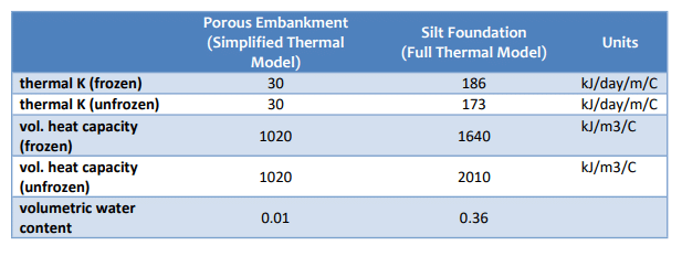
Table 1. Thermal properties for the embankment and foundation soils.
The latent heat of fusion for water is an important parameter in a heat flow analysis involving ground freezing (Set | Units and Scale). The default value is 334,000 kJ/m3, which is representative of pure water. Goering (2000) specified a value of only 26,200 kJ/m3. The inclusion of latent heat effects in a heat transfer analysis produces a highly non-linear problem that requires special algorithms to prevent numerical oscillation (i.e. non-convergence). The reduction of the latent heat coefficient by over an order of magnitude would certainly promote convergence while altering the propagation of the freezing and thawing front in the foundation soil. The default value provided by TEMP/W was retained, which would naturally lead to some difference in the solution as compared to Goering (2000).
The steady-state analysis was completed by applying a pore-air pressure of 0 kPa to the top of the embankment and a temperature of -2°C to the bottom of the domain. The boundary conditions result in hydrostatic pore-air and temperature distributions.
The top of the embankment was simulated using a no-flow air boundary (i.e. no air boundary condition applied) to represent the negligible air hydraulic conductivity of asphalt. Goering (2000) simulated the side-slope using both a no-flow boundary condition and an air pressure boundary condition that obeyed a harmonic function. In this study, all sides of the domain were assumed impermeable and therefore modeled as a no flow boundary condition. As noted above, this condition represents coverage by high moisture content topsoil or snow cover during the winter months.
Goering (2000) used the N-factor approach to determine harmonic temperature functions that were representative of the temperature on the asphalt surface, side-slope, and native soil surface. The function was given by:
𝑇 = 𝐴 ‒ 𝐵𝑐𝑜𝑠(2𝜋(𝑡 ‒ 9)/365 )
where 𝑡 is the Julian Day Number, 𝐴 yearly mean temperature, and 𝐵 the amplitude of the harmonic function. The coefficient 𝐴 was set equal to 1.1, 2.7, and -1.9°C for the asphalt, side-slope, and native soil respectively. The coefficient 𝐵 was set equal to 26.1, 20.9, and 10°C for the asphalt, side-slope, and native soil, respectively. Figure 5 shows the harmonic temperature functions along all three surfaces. The functions were defined over 365 days and the option to cycle (the function) was selected. Goering (2000) notes that the mean temperature of the native soil of – 1.9°C promotes permafrost while the mean temperatures of the embankment surfaces are above 0°C and therefore promote deterioration of the permafrost.
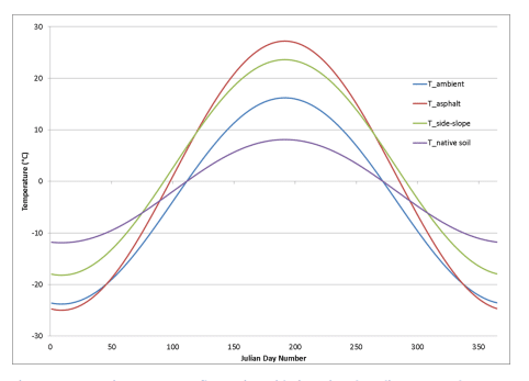
Figure 4. Harmonic temperature fluctuation with time given by Julian Day Number.
The left (symmetry) and right boundaries were considered adiabatic in the TEMP/W analysis. A geothermal ground heat flux of 5.2 kJ/day/m2 (0.06 W/m2) was applied to the bottom of the domain.
Goering (2000) simulated the harmonic temperature distribution cycling for 25 years using time steps of 0.25 days. The purpose of the long simulation time was to obtain the periodic annual cycles of air flow and heat transfers that govern the conditions of the foundation soil. Goering (2000) presented results for the last year of the simulation on August 1 and February 1, which are the periods during the cycle at which conduction and convection dominate the heat transfer, respectively.
For demonstrative purposes, the convective heat flow analysis was only solved for two cycles of the thermal boundary functions. The duration of the convective analysis was therefore specified as 730 days. The Julian Day Numbers for August 1 and February 1 dates on the 1st and 2nd cycle of the simulation are 214/579 and 397/762, respectively. These specific elapsed times could be entered into the list that appears at the bottom of the Time tab, making data available on these days for graphing and contouring. The transient analysis needed to be initiated at a time that provided boundary temperatures that were similar to the initial ground temperature of -2°C. The temperatures of the boundary functions on March 31 (Julian Day # 91) ranged between about -1°C and -3.5°C (Figure 4); consequently, Day 91 was selected to initiate the transient analysis. This was facilitated by specifying a starting time of 90 days and duration of 1 day in the steady-state analysis (Figure 2), which forces the start time of the transient analysis to be Day 91.
The transient analysis was completed using 1 day steps. Smaller times steps of 0.25 days were also used to promote convergence during freeze/thaw cycles; however, the simulated results were negligibly different, so the analysis was not retained.
Results and Discussion
Goering (2000) provides an insightful discussion on the physical process operating to promote convective cooling. Only a brief summary of some of the highly relevant results are provided. As will be apparent, the results of the simulations are comparable despite some important difference between the simulations that should be noted at the onset, including:
- An order of magnitude difference in the latent heat of fusion for the foundation soil;
- Potential discrepancies in the air hydraulic conductivity of the porous embankment;
- Differences in time stepping strategies;
- Differences in the physics (partial differential equations), element types (meshing), and
integration order; - Differences in the algorithms required to handle latent heat effects; and,
- Goering (2000) simulated 25 cycles, but the results presented here are from only 2 cycles
Figure 5 compares the simulated convective cells on the saved time nearest to February 1 of the 2nd cycle (Julian Day # 762). Two large and dominate convective cells develop below the pavement surface of the Goering (2000) simulation, circulating the air in clockwise (centerline) and counter-clockwise directions. Goering (2000) calculated a mean velocity of 8.8 m/hr (Figure 5). A mean velocity of about 7 m/hour was produced by the GeoStudio simulation, which is in reasonable agreement considering the aforementioned discrepancies. The average was calculated in a spreadsheet by using Draw | Graph to obtain the air x-y-fluxes for all nodes within the region comprising the embankment. Again, it is noted that the discrepancies in the convective cells are a by-product of the simulation time. For example, the two distinctive convective cells develop in the 3rd and 4th cycles of a 4 year simulation.
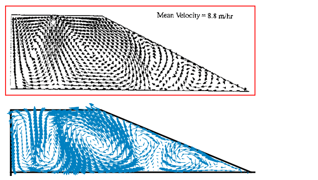
Figure 5. AIR/W pore-air flux vectors (bottom) on February 1 of the 2nd cycle (Julian Day # 762) as compared to Goering (2000) after 25 cycles.
Goering (2000) notes that a critical temperature difference between the upper and lower boundaries must be exceeded for natural convective cells to develop. Convection occurs during the portion of the climate (temperature) cycle when there is a relatively low temperature at the surface compared to the warmer temperature near the base of the embankment. Figure 6 shows the temperature history at a node at the interface between the embankment and foundation as compared to the harmonic temperature function applied to the pavement surface. The convective air cells initiate circulation as early as about Julian Day Number 321 and 681 on the 1st and 2nd cycles when the base of the embankment is around 0°C. The asphalt surface had not yet reached its coldest point when the critical temperature difference was exceeded.
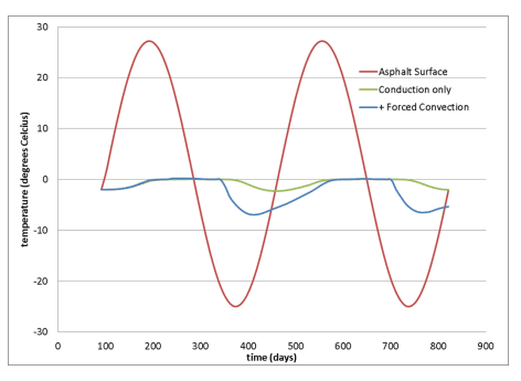
Figure 6. Temperature history at the interface between the embankment and foundation along the line of symmetry as compared to the harmonic asphalt temperature.
Figure 7 shows the temperature plume structures that develop due the large air fluxes within the convective cells. The pattern of temperature contours matches the pore-air convective cells. The cells form during the winter months due to the unstable pore-air density stratification within the embankment (Goering, 2000). The plume beneath the driving lane simulated by GeoStudio in the 2nd cycle compares well with Goering (2000) after the 25th cycle as is evidenced by the -16°C and -14°C contours. The -4°C contour is also at a nearly identical location within the foundation soil. Goering (2000) notes that the influence of the plume is evidenced by the fact that the -4°C contour has penetrated almost as deep beneath the centerline as it has beneath the native land surface, despite the 2.5 m of coarse overburden.
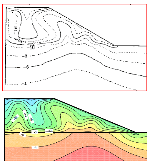
Figure 7. AIR/W temperature contours (bottom) on February 1 of the 2nd cycle (Julian Day # 762) as compared to Goering (2000) after 25 cycles.
During the summer months, the pore-air density gradient is more stable and the air fluxes are negligible. Conduction dominates the heat transfer process and temperature contours are relatively horizontal within the embankment (Figure 8). Goering (2000) notes that the depth of thaw has not progressed as deep into the foundation soil beneath the embankment than it has beneath the native land surface.
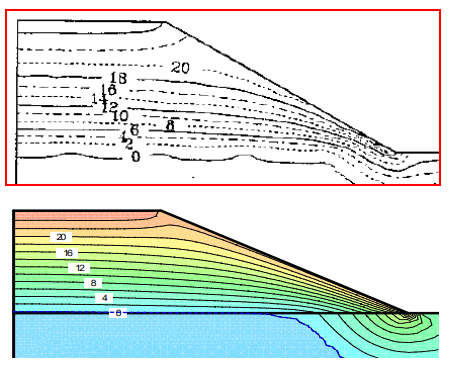
Figure 8. AIR/W temperature contours (bottom) on August 1 of the 2nd cycle (Julian Day # 579) as compared to Goering (2000).
Figure 9 shows the measured temperatures within the test embankment on August 1 and February 1. The external conditions imposed on the embankment deviated considerably from those simulated. Despite these variations, the numerical simulations reproduce the temperature patterns and help elucidate the mechanisms controlling the potential for thaw of the permafrost. The measured temperatures clearly reflect the existence of convective activity within the embankment during the winter months and conduction dominant heat transfer during the summer months (Goering, 2000).
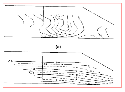
Figure 9. Measured temperature contours on February 1 and August 1 (Goering, 2000).
Summary and Conclusions
AIR/W can be used in combination with TEMP/W to simulate passive cooling within coarse materials due to the development of convective cells. Passive cooling can prevent thaw of underlying permafrost, thus eliminating thaw settlement (Goering, 2000). Goering (2000) also notes that natural convection in coarse material can cause enhanced seasonal freezing beneath embankments and, therefore, exacerbate problems with frost heave in foundation soils for certain climates. That is to say, passive cooling is only advantageous in some (cold) climates.
References
Goering, D.J. and Kumar, P. 1996. Winter-time convection in open-graded embankments. Cold Regions Science and Technology, 24, 57-74.
Goering, D.J., 1998. Experimental investigation of air convection embankments for permafrost-resistant roadway design. Proceedings of the 7th International Conference on Permafrost, Yellowknife, NWT, 319-326.
Goering, D.J. 2000. Passive cooling of permafrost foundation soils using porous embankment structures. American Society of Mechanical Engineers (ASME), Heat transfer Division, 366-5, 103-111.