Oasis montaj: redesigned filtering (Remote Roundup 2021)

Learn how you can save time and with our updated and interactive filtering in Oasis montaj. We will show you a redesigned 1D and 2D filtering workflow performing industry-standard filters and transforms.

Overview

Video Transcript

[00:00:00.618](ethereal music)

[00:00:10.120]<v ->Hello, good morning.</v>

[00:00:10.953]Good afternoon to everyone in attendance.

[00:00:14.020]Today, we’re going to be looking at redesigned filtering

[00:00:16.630]workflows that we’ve introduced into the latest version

[00:00:19.460]of Oasis montaj version 9.9.

[00:00:24.010]We’re going to be working with some real world data,

[00:00:26.280]and tackling some real world problems today.

[00:00:28.820]So I hope you enjoy today’s demonstration.

[00:00:31.580]So just a quick introduction for myself.

[00:00:35.160]My name is Geoff Plastow,

[00:00:36.420]and I’m a Senior Geophysicist here at Seequentt,

[00:00:39.110]and I’m currently based in Vancouver, British Columbia.

[00:00:43.060]As you can imagine from the title of this webinar,

[00:00:46.330]we have redesigned some of the key filtering workflows

[00:00:49.480]inside of Oasis montaj.

[00:00:51.800]This updated filtering process is now much more visual,

[00:00:55.610]much more interactive and much more intuitive.

[00:00:59.250]In turn, this is going to make you more efficient

[00:01:01.410]with your time and takes a lot of the guesswork,

[00:01:04.020]and trial and error involved in the filtering process.

[00:01:07.710]So now you could focus on understanding,

[00:01:10.100]and interpreting the data.

[00:01:13.320]So before we get too far into today’s conversation,

[00:01:16.800]perhaps I can mention why we might even want to filter

[00:01:19.500]our data to begin with.

[00:01:21.500]For those attending,

[00:01:22.810]feel free to use the chat panel,

[00:01:24.500]to type in some other reasons why you might want to filter

[00:01:27.260]your own data.

[00:01:29.580]Some of the most common reasons why we might want to filter

[00:01:32.140]our data is to accentuate or to highlight

[00:01:35.020]part of a geophysical or geological response,

[00:01:38.350]or to perhaps suppress something that we see in the data.

[00:01:42.060]For example,

[00:01:43.200]we may want to suppress systematic noise or random noise,

[00:01:47.590]and accentuate subtle geological and geophysical anomalies.

[00:01:52.280]I’m going to jump into Oasis montaj now.

[00:02:03.680]In Oasis montaj,

[00:02:05.210]part of the filtering process allows us to perform

[00:02:07.830]transforms on our data as well.

[00:02:10.410]We can transform a very simple magnetic datasets

[00:02:13.570]like we’re looking at now

[00:02:15.454]into something more interpretable,

[00:02:17.410]and perhaps a higher order deliverable.

[00:02:19.900]This is what we’re going to do today.

[00:02:22.420]So let’s have some fun and let’s get to work on an airborne

[00:02:25.150]magnetic datasets.

[00:02:28.100]So here we are in the latest version of Oasis montaj

[00:02:31.110]released in November of 2020.

[00:02:33.910]We’re going to start with the Geosoft database

[00:02:36.120]containing some airborne magnetic data.

[00:02:39.180]So on the right side of the screen,

[00:02:40.690]we see our Geosoft database, it’s a very simple database.

[00:02:44.430]We have our location information, Eastern and Northern.

[00:02:47.820]We have our radar altimeter,

[00:02:49.320]which is the sensor height above the surface of the earth.

[00:02:52.340]And we have our final magnetic data.

[00:02:55.110]And here we see a profile of our magnetic data in red.

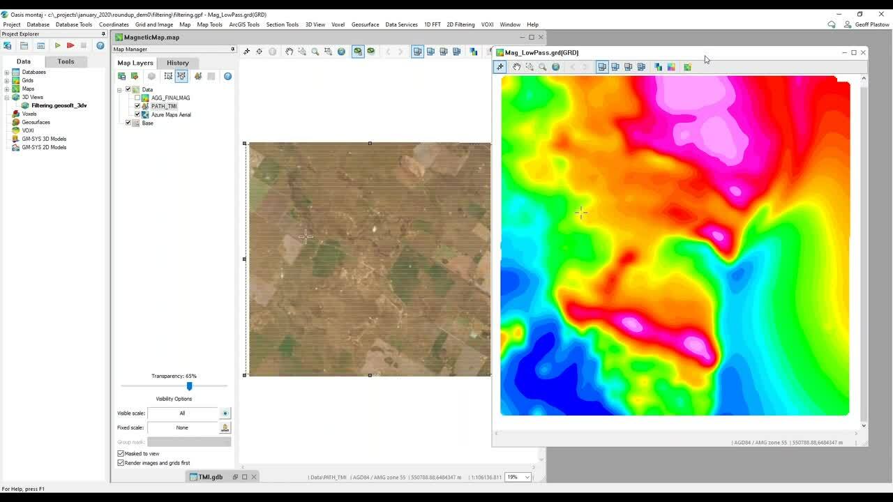
[00:02:59.690]On the left-hand side of the screen,

[00:03:02.010]we see a map containing the same data gridded.

[00:03:07.220]The areas in red or pink represent areas of a high magnetic

[00:03:10.760]intensity and the areas that are cool or blue in color

[00:03:14.190]represent areas of low magnetic intensity.

[00:03:18.980]Now all geophysical projects have their challenges.

[00:03:22.890]And of course, this one is no exception.

[00:03:26.670]Below this image,

[00:03:27.870]we’re looking at some satellite imagery

[00:03:29.760]over the survey area,

[00:03:31.370]and we can see all of these specs and dots

[00:03:34.580]over the survey area, and they represent culture.

[00:03:37.860]They represent drill pads,

[00:03:39.360]they represent drill casings and shacks,

[00:03:41.770]and other metallic objects.

[00:03:45.300]And our airborne geophysical survey has picked up

[00:03:48.130]all of those items and we can see them in our dataset

[00:03:51.430]as these very small magnetic anomalies.

[00:03:54.950]And our first challenge that we’re going to tackle today

[00:03:57.480]is we’re going to try to separate or remove these small

[00:04:00.810]magnetic features from our magnetic dataset.

[00:04:04.230]So we’re going to use the 1D FFT filtering capability

[00:04:08.290]in Oasis montaj to do that.

[00:04:11.400]So I’m going to click 1D FFT and 1D filtering.

[00:04:17.410]So right off the bat where we can see our redesign

[00:04:20.460]1D filtering menu, this is completely resizable,

[00:04:24.800]and I’m going to make it full screen

[00:04:26.150]so everyone can see it clearly.

[00:04:28.860]The 1D FFT filtering is divided into three panels.

[00:04:33.370]At the top, we have our power spectrum,

[00:04:36.460]which we can look at wave length or wave number.

[00:04:40.320]And as a quick reminder,

[00:04:41.760]the power spectrum is a 48 transform of our magnetic data.

[00:04:46.470]And we’re looking at it in the energy space.

[00:04:49.150]So we’re looking at wave length or wave number

[00:04:52.280]on the horizontal scale.

[00:04:53.640]And we’re looking at energy on the top scale,

[00:04:56.790]on the vertical scale.

[00:04:59.110]The center panel gives me a nice preview

[00:05:02.400]of our magnetic data.

[00:05:05.400]And at the bottom here, we have our filter design panel.

[00:05:11.000]So I’m going to select the database channel

[00:05:13.350]that we want to filter.

[00:05:14.410]We’re going to filter our magnetic data,

[00:05:16.820]and we’re going to provide an output channel.

[00:05:19.400]I’m going to call this our low pass filter data.

[00:05:23.230]And here I can design the first filter that we can apply.

[00:05:26.950]I’m going to apply a low pass filter,

[00:05:29.920]and here I can adjust the filter design properties.

[00:05:34.600]And these are in our ground units where it’s around meters.

[00:05:37.750]So I can apply,

[00:05:38.670]let’s say a 200 meter filter and right off the bat,

[00:05:43.280]we can see our power spectrum window updates.

[00:05:47.610]In blue, we see our filter response.

[00:05:50.950]We can see our original data here in the frequency domain

[00:05:54.880]of our original spectrum.

[00:05:56.730]And we see the filtered spectrum as well.

[00:05:59.750]We can also see a preview of the filtered response.

[00:06:04.020]I’m just going to make it a little bit larger.

[00:06:07.520]So you can see here that we’ve made a little dent

[00:06:09.780]in these cultural anomalies, but not much.

[00:06:12.960]So we can simply just increase this number automatically.

[00:06:17.640]And I hit enter and the filter updates,

[00:06:20.970]the filter of response updates in real time,

[00:06:23.350]and we see a preview of our filtered response right away.

[00:06:27.780]So this takes a lot of guesswork out of designing a filter.

[00:06:31.080]We can see it in the frequency domain.

[00:06:32.950]We can see a live preview of our data,

[00:06:35.620]and we can automatically adjust and fine tune things.

[00:06:38.870]That’s how we find the ideal filter settings.

[00:06:41.800]Once we’re ready, we can click okay.

[00:06:43.980]And we can apply this filter to our database.

[00:06:47.670]I’m just going to display the low pass filter data

[00:06:53.370]on top of our original dataset,

[00:06:56.120]so we can examine it a little bit more clearly.

[00:06:59.240]So we can see,

[00:07:00.073]we did a pretty good job of removing these small cultural

[00:07:03.480]anomalies, at the same time,

[00:07:06.060]doing our best to maintain the geologic response

[00:07:08.950]of the project area.

[00:07:11.600]The next thing I’m going to do is I’m just going to create

[00:07:13.560]a quick grid of our low pass filter data.

[00:07:20.210]So now we have an updated image of our culture removed

[00:07:24.880]magnetic data.

[00:07:27.150]So let’s go ahead and check out some of the 2D filtering

[00:07:30.400]capabilities inside of Oasis montaj.

[00:07:34.740]As you may have noticed,

[00:07:35.800]we’ve renamed our mag map extension 2D filtering.

[00:07:40.080]We’ve done this to address the more broadly applicable

[00:07:43.160]2D filtering capabilities of the extension.

[00:07:47.070]So let’s go ahead and start filtering our magnetic data.

[00:07:54.290]Our input here is going to be our low-pass grid

[00:07:57.380]that we just created, and we’re going,

[00:08:00.100]the first filter we’re going to apply is going to be a first

[00:08:03.130]vertical derivative.

[00:08:05.250]This is a very common geophysical filter that is applied

[00:08:08.430]to accentuate near surface information,

[00:08:11.800]and to accentuate lineaments contacts and faults,

[00:08:14.607]and the dataset.

[00:08:17.160]I’m going to provide the name for the output grid,

[00:08:20.160]and a name for our filter design file.

[00:08:23.040]Once we’re ready, I can click, edit or create a filter.

[00:08:31.720]We’re met with a new redesigned 2D filtering window.

[00:08:36.520]Again, this is completely customizable and can be resized.

[00:08:40.500]I’m going to go ahead and make it full screen.

[00:08:44.120]Inside of this, we can resize and rescale our windows.

[00:08:49.150]Let’s just talk a bit about what we’re looking at.

[00:08:52.670]In the top right-hand corner,

[00:08:54.220]we can see a grid of our magnetic data.

[00:08:56.820]We can see our coordinates and we can also see the value

[00:08:59.640]of our data.

[00:09:00.720]So here, we’re looking at nanoteslas.

[00:09:04.490]On the left-hand side here,

[00:09:05.950]again, we see a power spectrum of our input data.

[00:09:09.710]So again,

[00:09:10.970]this is the power spectrum or the Fourier transform

[00:09:14.470]of our input survey data.

[00:09:16.160]And we’re looking at it in the frequency domain.

[00:09:19.270]Like we can switch between wave length and wave number,

[00:09:22.060]if you’re comfortable in working on either of those

[00:09:24.760]formats.

[00:09:26.460]We can see our filter design here in blue.

[00:09:29.770]We can see our original input power spectrum in black,

[00:09:34.180]and the filtered spectrum here in red.

[00:09:38.370]If we want, we can resize this window,

[00:09:41.100]if we want to look at a specific part of the power spectrum.

[00:09:46.380]And again, we can resize these as we need.

[00:09:50.010]What’s great is we have a huge option,

[00:09:52.500]a huge list of filters that we can use to accentuate,

[00:09:55.940]and transform our data.

[00:09:57.770]The first filter I’m using is a regional residual separation

[00:10:01.530]filter.

[00:10:02.870]Here, we can assign the cutoff wavelength.

[00:10:06.130]If we want, we can just simply just click and scroll,

[00:10:09.180]and you’ll see that the filter is automatically updated

[00:10:12.120]in the power spectrum.

[00:10:13.640]And the result,

[00:10:15.200]the preview of the filter is updated in the bottom left-hand

[00:10:19.070]corner.

[00:10:20.010]This is so useful,

[00:10:21.550]and it takes out so much trial and error

[00:10:24.140]out of our filtering process.

[00:10:26.530]So we can simply adjust the filtering parameters

[00:10:29.450]to accentuate the geophysical or geological features

[00:10:33.280]that we’re interested in.

[00:10:35.180]We can quickly switch between low pass, high pass,

[00:10:38.660]and we can also stack our filters.

[00:10:40.990]We can apply multiple filters at once, which is very common.

[00:10:45.500]So I’m first performing a regional filter on our dataset,

[00:10:49.510]and now I’m performing a derivative

[00:10:51.540]in the vertical set direction.

[00:10:54.000]If I wanted to see what the other directions look like,

[00:10:56.180]I can simply flip between them and I can get an automatic

[00:11:00.510]preview of what those results look like.

[00:11:04.720]What’s nice is if I’m stacking my filters,

[00:11:07.270]I can see the previewed result of all of them combined,

[00:11:10.920]or I can see the individual results of the regional filter

[00:11:14.570]or just the derivative filter as they’re applied.

[00:11:18.240]Once I’m happy with the design of my filter,

[00:11:21.210]I can click, okay.

[00:11:23.620]And then, okay to create my filtered 1VD grid.

[00:11:29.990]And you can see from this result,

[00:11:31.430]we’ve accentuated some of the faults in this area,

[00:11:34.780]as well as some of the intrusive bodies

[00:11:37.000]that are sticking out.

[00:11:39.320]So let’s jump back in and run another filter.

[00:11:44.360]The next filter I’m going to run

[00:11:46.200]is a reduce to pole transform.

[00:11:50.720]So I’m just going to rename my grid here,

[00:11:54.520]and I’m going to edit my filter file.

[00:12:01.200]And again, we’re going to jump into our 2D filtering.

[00:12:05.200]So in case you didn’t know,

[00:12:06.690]reduction-to-pole or RTP is a transform,

[00:12:10.500]which removes the dependence of magnetic inclination

[00:12:13.230]from our magnetic data.

[00:12:16.280]RTP or reduction-to-pole is a transform that aims

[00:12:19.560]to remove any assymetry or distortion

[00:12:22.630]caused by magnetic inclination.

[00:12:25.230]This more or less results in anomalies

[00:12:28.250]above their magnetic sources.

[00:12:30.720]This is a pretty common transformant magnetic processing,

[00:12:34.120]and really eases some of the processes involved

[00:12:37.610]in interpretation.

[00:12:40.060]So I can go ahead and again, make this a full screen.

[00:12:44.400]We can see our power spectrum here on the left-hand side.

[00:12:47.420]We can see our original and our output grid.

[00:12:50.690]So to do an RTP transform,

[00:12:52.870]I can simply select this from our dropdown list.

[00:12:57.430]What’s great is all I have to do is enter

[00:12:59.460]in the survey date.

[00:13:01.870]So this is the date that the data was acquired.

[00:13:04.180]I can click calculate,

[00:13:05.750]and it will automatically calculate the inclination,

[00:13:08.990]and declination for this project area.

[00:13:11.820]And I can click, okay.

[00:13:13.580]And I can perform our reduction-to-pole

[00:13:16.230]on our magnetic data.

[00:13:18.810]So you can see that the 2D filtering,

[00:13:21.290]or redesigned 2D filtering extension really,

[00:13:25.620]really assist interpretation by allowing us to preview

[00:13:28.890]the result before re-filtering.

[00:13:30.630]And it takes a lot of the guesswork out of the process.

[00:13:35.070]What I’d like to show you next is our new matched filtering

[00:13:40.180]inside of our 2D filtering extension.

[00:13:44.580]So what is matched filtering?

[00:13:46.750]Matched filtering is a separation filter,

[00:13:49.680]or layer filtering process,

[00:13:51.810]which is a new addition to the latest version

[00:13:53.870]of Oasis montaj.

[00:13:56.100]Matched filtering gives us our first glimpse,

[00:13:59.300]or insight as to how our magnetic structure changes

[00:14:02.790]from near surface or short wavelength, to depth,

[00:14:06.860]long wavelength.

[00:14:08.450]It provides us some quick insights into the relationship

[00:14:11.430]between wavelength and equivalent source depth

[00:14:14.430]in our magnetic data.

[00:14:16.610]The aim of matched filtering is an attempt

[00:14:18.590]to isolate magnetic sources to an ideal layer

[00:14:22.050]at an equivalent depth.

[00:14:24.620]So in the matched filtering menu,

[00:14:27.220]we can see a similar window that we saw

[00:14:29.490]in our 2D filtering extension.

[00:14:31.630]We have our input magnetic data,

[00:14:33.600]which is the RTP grid that we just created.

[00:14:37.220]And we can see our power spectrum on the left-hand side.

[00:14:41.640]Again, we have the black line,

[00:14:43.820]which represents the original survey data,

[00:14:48.140]and we have our long wavelengths at left-hand side

[00:14:53.100]of the screen.

[00:14:53.933]This represents the deeper structure or deeper sources

[00:14:57.030]in our dataset.

[00:14:58.800]And on the right-hand side,

[00:15:00.040]we have our high-frequency content,

[00:15:02.540]or our near surface structure.

[00:15:05.410]And we can see a number of filters that have been applied

[00:15:09.580]to our data set.

[00:15:11.290]So I’m just going to zoom in to part of the spectrum.

[00:15:13.770]So we can little bit see our filters

[00:15:16.640]a little bit more clearly.

[00:15:18.690]So the first filter that we apply is a low pass filter.

[00:15:23.280]The last filter that we apply here is a high pass filter.

[00:15:27.570]And then for each of the equivalent depths

[00:15:30.200]that we are going to try to extract from our dataset,

[00:15:33.460]we provide a tapered band pass filter,

[00:15:37.100]so we can extract up to four equivalent depth.

[00:15:40.620]In this case,

[00:15:41.453]I have three and we can see the preview of them

[00:15:45.110]on the bottom right-hand corner of the screen.

[00:15:47.670]I can preview equivalent source depths at five kilometers.

[00:15:52.850]Here we are at two and a half kilometers,

[00:15:55.800]and then 1000 meters.

[00:15:58.680]And you’ll see, as I move here,

[00:16:01.060]the updated spectrum that we’re looking at is updated

[00:16:04.150]in the power spectrum window.

[00:16:09.060]I’m just going to resize this.

[00:16:11.600]If we want,

[00:16:12.433]we can interactively select an equivalent source depth

[00:16:15.580]from our window.

[00:16:16.800]I can click on this edit button and I can pick the depth

[00:16:20.010]on the spectrum.

[00:16:21.540]And it’s going to actually provide me some information

[00:16:25.480]about what depth we were going to pick.

[00:16:28.350]So if I wanted to extract something at around

[00:16:31.990]the 700 meter equivalent source depth layer,

[00:16:37.270]I can go ahead and just click that,

[00:16:39.410]and it’ll automatically update itself here.

[00:16:42.610]Once I’m ready to perform the separation filter,

[00:16:45.170]I can click, okay.

[00:16:46.880]And it will extract my matched grids.

[00:16:56.110]So we have our four filtered grids.

[00:16:58.270]Our first grade represents all of our high-frequency

[00:17:01.680]near surface structure.

[00:17:02.980]You can see it’s really extracting these near surface

[00:17:05.380]liniments and faults.

[00:17:08.240]Again, now here’s our one kilometer or sorry,

[00:17:10.930]our about 700 meter equivalent layer,

[00:17:15.200]our two and a half kilometer equivalent layer,

[00:17:18.020]and our five kilometer layer,

[00:17:19.670]which is really looking at our, some of our long wavelength,

[00:17:22.720]deep seated structures.

[00:17:26.350]So matched filtering makes a useful contribution,

[00:17:30.420]and enhancements to our magnetic data.

[00:17:32.617]And this example,

[00:17:33.810]it allows us to approximate and separate deep seated

[00:17:36.960]structure from near surface faults

[00:17:39.530]in our magnetic dataset.

[00:17:41.840]Matched filtering is incredibly useful in Oasis montaj,

[00:17:46.070]and part of our new addition to our 2D filtering toolkit.

[00:17:50.100]It provides fast qualitative understanding

[00:17:52.790]of the equivalent layers and the equivalent wavelengths.

[00:17:56.240]It provides us insights into the separation of deep seated

[00:18:00.160]magnetic structure and near surface magnetic responses.

[00:18:04.860]In all of our redesigned filtering workflows,

[00:18:07.710]they’ve become much more visual and intuitive to use.

[00:18:11.410]Instead of a lot of trial and error or blindly filtering

[00:18:14.040]your data,

[00:18:14.873]we can now see automatic previews of our filtered data.

[00:18:17.870]This is going to save us time and effort,

[00:18:19.830]and allows us to focus on bigger problems related

[00:18:22.500]to our exploration projects.

[00:18:28.270]So this concludes my demonstration this morning.

[00:18:31.620]Thank you very much for your time.

[00:18:34.069](ethereal music)