Oasis montaj: how to improve your understanding of an exploration project with magnetic data

Using open-source Geoscience data, we will illustrate how Oasis montaj can improve your understanding of an exploration project. This demonstartion will highlight some of the new magnetic interpretation tools within Oasis montaj. We will start with some fundamentals, 1D & 2D Filtering, then jump into Grid Texture Analysis, Magnetic Inverison and Self-Organizing Maps.

Get more from your data.

Overview

Video Transcript

[00:00:00.071]
(soft music)

[00:00:09.930]
<v Geoff>Hello, and good morning</v>

[00:00:11.420]
and good afternoon to everyone in attendance.

[00:00:14.250]
Welcome to a live presentation

[00:00:16.060]
at the 2021 PDAC Virtual Conference.

[00:00:21.100]
Thank you so much for joining today.

[00:00:23.590]
We’re going to be looking at Oasis montaj

[00:00:25.620]
and how to improve your understanding

[00:00:27.450]
of an exploration project with magnetic data.

[00:00:31.930]
So just a quick introduction.

[00:00:33.750]
My name is Geoff Plastow,

[00:00:34.583]
and I’m a senior geophysicist here at Seequent,

[00:00:37.940]
and I am currently based in beautiful

[00:00:39.920]
Vancouver, British Columbia.

[00:00:42.047]
I’ve been at Seequent for just about three years now,

[00:00:45.280]
but I’ve been using Oasis montaj for about 15 years.

[00:00:48.600]
I’ve had the opportunity to work with a wide variety

[00:00:51.120]
of geoscience and geophysics datasets,

[00:00:53.920]
everything applied to exploration, energy,

[00:00:57.130]
civil and environmental applications.

[00:01:00.000]
I should also mention on the webinar panel

[00:01:02.160]
and monitoring today, we have my colleagues,

[00:01:04.910]
Adriana Carbone, and Kanita Khaled.

[00:01:09.930]
Before we get too far into our discussions today,

[00:01:12.610]
I just have a quick statement

[00:01:13.850]
of confidentiality and disclaimers.

[00:01:16.500]
I’m not going to read it to you,

[00:01:17.800]
but I’m just going to leave it here

[00:01:18.950]
for a moment for you to digest.

[00:01:22.230]
The good thing or the great news

[00:01:23.920]
about today’s presentation

[00:01:25.330]
is that everything I’m showing is available

[00:01:27.270]
in the current release of Oasis montaj version 9.9

[00:01:31.610]
and it’s available to all maintained

[00:01:33.370]
and subscription customers.

[00:01:38.270]
So what are we going to look at today?

[00:01:40.380]
Today’s focus is an early stage

[00:01:42.110]
greenfields exploration project.

[00:01:44.420]
Our objective will be to take a public domain data

[00:01:47.160]
and extract more information

[00:01:50.037]
from the magnetic data

[00:01:51.700]
to try to vector our exploration efforts

[00:01:53.820]
to the most prospective areas

[00:01:55.330]
within the project area.

[00:01:57.040]
So what are we actually going to look at?

[00:01:58.870]
We’re going to look at some open geoscience data,

[00:02:01.120]
where to get it and how to quickly get it

[00:02:02.660]
and integrate it into your project.

[00:02:04.690]
We’re going to look at a new Multi-Trend Gridding algorithm

[00:02:07.390]
available in Oasis montaj.

[00:02:09.560]
We’re going to look at some 2D filtering or data transforms

[00:02:12.560]
that we can apply to magnetic data

[00:02:14.160]
to squeeze more out of it.

[00:02:16.230]
We’re going to do some grid texture analysis.

[00:02:18.410]
So we’re going to extract the fabric from our magnetic data

[00:02:21.017]
and we’re going to create a structural complexity map.

[00:02:24.030]
Then after this, we’re going to take a look

[00:02:25.330]
at some magnetic inversions

[00:02:26.880]
and how they can also improve our insights

[00:02:29.200]
into our project area.

[00:02:35.060]
So just before I get going,

[00:02:36.420]
just a couple of acknowledgements,

[00:02:38.260]
the dataset we’re looking at today,

[00:02:39.850]
it’s a public domain dataset.

[00:02:42.130]
The data is available on the Natural Resources Canada’s

[00:02:45.640]
Geoscience Data Repository.

[00:02:48.460]
The link is here

[00:02:49.880]
and this data repository is powered

[00:02:52.730]
by Seequent DAP technology.

[00:02:55.220]
So for those who are using Oasis montaj and Target,

[00:02:58.880]
you could access this data and a huge wealth of geoscience

[00:03:02.130]
information via Seeker.

[00:03:04.420]
The name of today’s dataset,

[00:03:05.780]
or what it’s called is the Southern Glennie project.

[00:03:08.140]
It was collected in late 2019

[00:03:10.230]
and early 2020 by Geotech.

[00:03:13.010]
And for those who are aware,

[00:03:14.780]
it is a VTEM max system.

[00:03:21.870]
Just a quick comment about the project area,

[00:03:25.900]
where the project area is located in Northern Saskatchewan.

[00:03:28.610]
So just to locate ourselves,

[00:03:29.850]
my apologies for the quality of these images

[00:03:31.590]
they were just taken from the report.

[00:03:33.830]
This is Saskatchewan, we have Lloydminster, Flin Flon,

[00:03:36.770]
and we have La Roche, and this is Lac La Loche here.

[00:03:40.900]
The crew is situated in Lac La Loche,

[00:03:42.770]
and this is the actual project area.

[00:03:46.710]
The geophysical survey data that was collected

[00:03:49.220]
was airborne magnetic and time-domain electromagnetic data.

[00:03:53.920]
There was a total of 6,500 line kilometers that covered

[00:03:58.340]
approximately 1,100 square kilometers.

[00:04:02.150]
And just for perspective, this is 80 kilometers end-to-end.

[00:04:05.360]
So it’s a pretty large exploration area.

[00:04:10.580]
So why are we talking about magnetic data today?

[00:04:13.740]
Well, in Canada, we’re so lucky.

[00:04:16.550]
Most of Canada is covered with high quality magnetic data

[00:04:20.030]
and Natural Resources Canada

[00:04:21.520]
and the various provincial governments and organizations

[00:04:23.880]
are always adding new datasets into the mix,

[00:04:26.850]
just like this one.

[00:04:28.960]
But really why magnetic data?

[00:04:31.010]
Well magnetic data is a cost-effective way

[00:04:34.960]
to map geological and geophysical environments.

[00:04:42.440]
It can be acquired on the ground,

[00:04:44.840]
it can acquired in the air

[00:04:46.320]
through airplanes, helicopters, UAVs,

[00:04:47.860]
and it could also be collected in marine environments.

[00:04:50.180]
So pretty much anywhere on earth

[00:04:51.830]
and it’s very cost-effective.

[00:04:54.680]
Magnetic data ultimately allows us explorers,

[00:04:57.500]
geoscientists to map and interpret geological features,

[00:05:00.580]
faults, dykes, contacts, intrusive bodies.

[00:05:03.860]
Magnetic data is a great structural mapping tool,

[00:05:06.640]
and it’s really one of the common denominators

[00:05:09.360]
in many exploration products.

[00:05:18.840]
Okay, I’m just going to jump into the application now.

[00:05:22.910]
I’m just going to jump into Oasis montaj.

[00:05:25.800]
I’m also just going to turn off my webcam

[00:05:27.220]
just to save a little bit of bandwidth.

[00:05:33.490]
So we’re actually going to start at the end.

[00:05:36.320]
We’re going to start at the end product

[00:05:37.918]
and then we’re going to kind of build towards it.

[00:05:40.390]
So what we’re looking at here is a 3D view

[00:05:44.100]
of our project area.

[00:05:46.820]
The overlay image in the background here,

[00:05:49.130]
this heat map, is a structural complexity heat map

[00:05:52.900]
that we’re going to create from our magnetic data.

[00:05:55.650]
The areas that are red or hot in color represent areas

[00:05:59.300]
that have a high structural complexity.

[00:06:02.300]
Then that means there’s lots of lineaments

[00:06:03.750]
and faults and folds that are intersecting each other

[00:06:05.940]
at a number of angles.

[00:06:08.620]
The black dots here represent all of the known mineral

[00:06:12.610]
occurrences within the project area.

[00:06:14.980]
I’ve downloaded these

[00:06:15.813]
from the government of Saskatchewan website,

[00:06:18.010]
and I’ve just imported them into Oasis montaj.

[00:06:20.790]
So predominantly in this area,

[00:06:23.170]
we have a number of known gold,

[00:06:26.320]
copper, pyrite mineralization.

[00:06:28.800]
We have a little bit of rare earth elements here as well,

[00:06:31.210]
and then as well,

[00:06:32.670]
gold on the Western side of the project area.

[00:06:35.950]
And underneath this,

[00:06:37.465]
we’ve done a magnetic inversion,

[00:06:43.010]
a magnetic vector inversion.

[00:06:45.690]
And these are some of the ISO surfaces from that inversion.

[00:06:51.000]
So this kind of what we are building towards.

[00:06:54.650]
So let’s jump into our project area.

[00:06:59.850]
So this red outline represents my area of exploration.

[00:07:05.470]
How do we get going?

[00:07:06.750]
Well, in Oasis montaj,

[00:07:08.287]
we can get into our data services menu.

[00:07:11.418]
And one of the first things I like to do is import

[00:07:14.460]
a satellite imagery through Bing Maps.

[00:07:18.070]
You’ll see that it loads very quickly,

[00:07:19.970]
and it just gives us a nice foundation base map,

[00:07:23.981]
for the project area.

[00:07:26.730]
After this, I can jump into Seeker.

[00:07:29.040]
And once I click the Seeker button,

[00:07:31.540]
this little pop-up is going to appear

[00:07:33.690]
and it’s grabbed the corner points of my map

[00:07:37.250]
or my area of interests,

[00:07:38.640]
my area that I’m exploring,

[00:07:40.620]
and it’s drawn this red box here.

[00:07:43.770]
I can resize it.

[00:07:45.150]
This is an area that I’m going to search

[00:07:47.340]
for public domain geoscience data.

[00:07:50.490]
Once I’m ready to click Search,

[00:07:52.960]
I can click the Results button.

[00:07:55.180]
So we can see that I’m connected

[00:07:57.060]
to the Natural Resources Canada Geoscience data portal.

[00:08:01.770]
There’s a huge variety of public domain data

[00:08:04.520]
that’s available across the country.

[00:08:07.190]
There’s also a number of other public domain

[00:08:09.160]
geoscience servers, including the Geosoft DAP Server

[00:08:11.880]
that serves a high resolution,

[00:08:14.220]
topography, magnetics and gravity information.

[00:08:17.750]
In this case, I’m just going to jump into the magnetics.

[00:08:20.350]
Radiometrics EM folder, jump into surveys

[00:08:23.900]
and here’s our project area.

[00:08:26.797]
And we can see a large number of survey deliverables.

[00:08:30.920]
I can click on a product I’m interested in.

[00:08:33.150]
I’ll get a quick preview of it.

[00:08:34.800]
And when I’m ready, I can just click Download,

[00:08:36.880]
and then download it to my project.

[00:08:40.570]
So right now my computer is reaching out

[00:08:42.260]
to the Natural Resources Canada’s server

[00:08:44.700]
and it’s downloaded

[00:08:47.910]
the total magnetic field data directly into my project.

[00:08:52.000]
It’s geo-referenced correctly.

[00:08:55.040]
So I don’t have to worry about referencing my data.

[00:09:00.340]
So one of the most important things

[00:09:02.950]
that we do in geophysics is visualizing

[00:09:07.910]
the data that we’ve collected.

[00:09:10.190]
And we call this technique gridding.

[00:09:14.281]
Gridding, it’s such an important thing,

[00:09:15.630]
but we don’t talk about it a lot.

[00:09:18.000]
It’s one of the key deliverables

[00:09:19.360]
that we provide our colleagues, our clients, our management,

[00:09:22.760]
and it’s really how we visualize our data.

[00:09:26.150]
Now, what are the challenges that we have

[00:09:28.180]
with magnetic data and geophysical data

[00:09:33.000]
is being able to honor the data

[00:09:37.290]
and honor the geological information

[00:09:40.170]
that we’re collecting or mapping.

[00:09:43.350]
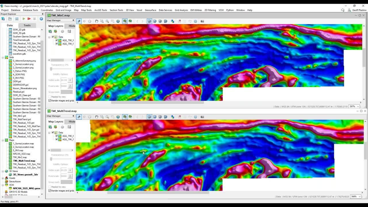
And I’m just going to show you just a quick example.

[00:09:47.570]
On the top of the screen here,

[00:09:48.840]
we have a grid of this very data we’re looking at

[00:09:53.080]
that was created

[00:09:54.540]
using the minimum curvature gridding technique.

[00:09:58.290]
The minimum curvature gridding technique

[00:09:59.810]
is a great technique.

[00:10:01.070]
It’s been around for a while,

[00:10:02.200]
it’s really fast, it’s robust,

[00:10:04.270]
it allows us to visualize data really quickly.

[00:10:06.650]
But one of the challenges that has is

[00:10:09.790]
it doesn’t allow us to enforce trends in the data.

[00:10:15.410]
So you can see that this magnetic dataset

[00:10:17.360]
has a lot of magnetic lineaments,

[00:10:18.971]
that are striking at different directions.

[00:10:22.530]
We have some east-west trending information.

[00:10:25.600]
We have some that are oblique to the survey lines.

[00:10:29.050]
Some that are perpendicular to the survey lines.

[00:10:31.590]
We have some circular features,

[00:10:33.870]
really minimum curvatures struggles a little bit with this,

[00:10:35.627]
and we can see some of this rippling

[00:10:37.560]
or broader nudging effects in minimum curvature data.

[00:10:42.580]
With the latest release of Oasis montaj 9.9,

[00:10:46.130]
we’ve included a new gridding technique

[00:10:48.300]
called the Multi-Trend Gridding technique.

[00:10:50.720]
And what this does

[00:10:51.600]
is it seeks out trends in your geophysical data,

[00:10:55.200]
and it tries to better honor that data by connecting them.

[00:11:00.750]
The great news is we don’t need to insert a specific trend

[00:11:04.540]
or strike direction.

[00:11:07.990]
The algorithm will simply do this for you.

[00:11:10.250]
So on the bottom here,

[00:11:11.350]
we have an image of the multi-trend gridded dataset.

[00:11:14.063]
This is the exact same dataset,

[00:11:16.510]
gridded at the same cell size.

[00:11:18.530]
So we don’t see a lot of this

[00:11:20.180]
sort of like broader nudging effects

[00:11:22.120]
or the string of pearls or rippling that we see

[00:11:25.420]
in minimum curvature gridding techniques.

[00:11:28.860]
So just to really highlight this,

[00:11:33.470]
if we try to work with this data,

[00:11:36.140]
the minimum curvature data,

[00:11:36.973]
and we try to do some data transforms,

[00:11:39.060]
let’s say we try to do a very simple

[00:11:40.840]
first vertical derivative.

[00:11:43.630]
Okay, so this broader nudging and rippling effect

[00:11:46.370]
really kind of stands out

[00:11:47.790]
and especially structure that’s oblique to the survey line.

[00:11:51.880]
When we use the Multi-Trend Gridding technique,

[00:11:55.600]
we can really preserve our efforts

[00:11:58.410]
and the hard work that we’ve done to collect process

[00:12:01.208]
and reduce the data.

[00:12:04.430]
And when we do higher order products

[00:12:06.390]
and we do derivatives, transforms,

[00:12:09.170]
we really eliminate some of these

[00:12:10.700]
sort of gridding artefacts from the data.

[00:12:12.500]
So if you are working

[00:12:13.660]
with potential fields geophysical data,

[00:12:15.780]
I would certainly recommend you

[00:12:17.080]
and your team check out the latest edition

[00:12:20.070]
of Multi-Trend Gridding,

[00:12:24.060]
on your magnetic dataset and just compare for yourself.

[00:12:29.460]
So I’ve already mentioned,

[00:12:30.970]
and we’re already looking at some data transforms.

[00:12:35.140]
So let’s take a look at

[00:12:36.950]
the new 2D Filtering tool within Oasis montaj.

[00:12:41.082]
One of the most common things

[00:12:42.150]
that we can do with magnetic data are transforms.

[00:12:45.180]
So we can take our total magnetic intensity data

[00:12:48.490]
and transform it into a higher order,

[00:12:50.910]
more valuable interpretation product.

[00:12:56.000]
So the first thing I’m going to do is click 2D Filtering,

[00:12:58.760]
then MAGMAP Filtering.

[00:13:00.020]
I’m going to provide it my total magnetic intensity,

[00:13:04.180]
multi-trend grid.

[00:13:05.500]
That was the grid that we were just looking at here.

[00:13:08.600]
And what we’re going to do

[00:13:09.590]
is we’re going to do just a first vertical derivative,

[00:13:12.590]
and I’m going to just click Create Filter.

[00:13:16.810]
What’s great about this tool

[00:13:18.470]
is that it is completely interactive.

[00:13:23.760]
So on the top right-hand corner here,

[00:13:25.550]
we have a map of our total magnetic intensity

[00:13:28.350]
across the survey area.

[00:13:29.970]
The areas that are pink or hot in color

[00:13:31.830]
represent the areas of a high magnetic intensity.

[00:13:34.660]
The areas that are blue or cold

[00:13:36.100]
represent an area that has a low magnetic intensity.

[00:13:39.610]
This is our data, and we can move around in here.

[00:13:41.840]
We can see the coordinates

[00:13:43.350]
and the values where I hover over.

[00:13:45.660]
As we move into the left-hand side of the screen,

[00:13:47.770]
we see a power spectrum of our data.

[00:13:50.400]
This is incredibly useful

[00:13:52.820]
if you are going to be applying filters to your data.

[00:13:56.360]
So let’s go ahead and do that.

[00:13:58.610]
The first filter I’m going to apply,

[00:14:00.700]
you’ll see once I click this,

[00:14:01.533]
I have a huge list of filters that I can apply.

[00:14:04.330]
Each one sort of has its own purpose.

[00:14:06.420]
For the sake of today’s presentation,

[00:14:08.430]
I’m not going to go through all of them obviously,

[00:14:10.610]
but I’m just going to focus on one of them

[00:14:12.280]
that I’d like to use,

[00:14:13.113]
it’s called the Gaussian regional residual filter.

[00:14:17.210]
The second I select this filter, a few things happen.

[00:14:20.940]
We see our original power spectrum here in black,

[00:14:23.620]
and we can automatically see

[00:14:24.860]
the filtered power spectrum in red.

[00:14:27.090]
We can also see the filter response here in blue.

[00:14:31.030]
What’s even better is that we have an automatic preview

[00:14:34.490]
of our filtered results.

[00:14:36.970]
So if we want, we can make changes to our filter.

[00:14:39.620]
We can make this a low pass filter.

[00:14:41.950]
We can adjust the filter cutoff wavelengths,

[00:14:45.590]
and we can really kind of play an experiment with our data

[00:14:50.950]
unlike we’ve been able to before.

[00:14:54.370]
So I’m just going to apply a 1, 500 meter wavelength cutoff,

[00:14:59.660]
and remember I’m going to apply it as a high pass.

[00:15:02.980]
And what this is doing is passing through

[00:15:05.740]
all of the short wavelength and near surface content.

[00:15:10.050]
And you can see that we’re extracting a lot more texture

[00:15:13.360]
and a lot more fabric from our magnetic data.

[00:15:17.250]
If we want to do even more,

[00:15:18.930]
I can add another filter so we can stack our filters

[00:15:22.240]
and run them sequentially.

[00:15:24.250]
So now I’m going to do a derivative.

[00:15:27.260]
So what we’re looking at here

[00:15:29.080]
is now the sequential application of the residual filter

[00:15:33.433]
and the derivative filter.

[00:15:35.710]
What’s great is I can look at a single one of these,

[00:15:38.740]
if I want to interrogate a specific area,

[00:15:42.080]
I can zoom in if I want,

[00:15:44.827]
I can zoom into an area of interest

[00:15:50.010]
and I can look at the derivative product,

[00:15:52.190]
or I can look at them combined.

[00:15:54.870]
When I’m ready, I can just click Okay,

[00:15:57.540]
and create that product.

[00:16:01.267]
And the whole process runs pretty quick.

[00:16:02.900]
Again, this is a pretty large project area.

[00:16:06.630]
So now we’ve created a higher order interpretation product.

[00:16:10.730]
We’ve stripped away some of the deeper structure,

[00:16:12.980]
we’re focusing on near surface structure.

[00:16:15.810]
We’ve really highlighted all the lineaments

[00:16:18.210]
in this dataset,

[00:16:19.043]
and we’re getting a lot more of the fabric

[00:16:20.910]
which is going to be useful in our next step.

[00:16:25.280]
So the next thing that we’re going to do

[00:16:26.920]
is we’re going to do some grid texture analysis.

[00:16:30.960]
So inside of Oasis montaj,

[00:16:32.610]
there’s an extension called the CET Grid Texture Analysis.

[00:16:36.190]
And what this allows us to do is extract the fabric

[00:16:39.650]
and lineaments from our magnetic data.

[00:16:43.260]
So we have a number of options.

[00:16:44.670]
We can select the highs or the lows,

[00:16:46.850]
the peaks and the troughs,

[00:16:48.030]
or perhaps we’re interested in the edges,

[00:16:50.130]
the contacts of the magnetic structure.

[00:16:53.120]
Following this, we have a number of ways to refine this.

[00:16:56.450]
So we can say we’re only interested

[00:16:58.800]
in lineaments in the Northwest direction

[00:17:00.630]
or the South direction.

[00:17:02.270]
We can do some thresholding.

[00:17:03.600]
So maybe we want to say,

[00:17:04.433]
we only want lineaments of a certain length.

[00:17:07.450]
Maybe we only want lineaments that are major,

[00:17:11.030]
so of a certain amplitude.

[00:17:13.240]
So we can really do some quality control and clean up

[00:17:17.240]
some of the structure.

[00:17:19.380]
So the grid that I’m showing you now,

[00:17:21.670]
this pinkish-blue grid is the extracted fabric,

[00:17:27.810]
the extracted lineaments from our magnetic datasets, right?

[00:17:32.240]
So we’ve extracted so much more information

[00:17:34.750]
than just working

[00:17:36.120]
with just a total magnetic intensity dataset.

[00:17:40.770]
And what’s great is we can now display this information

[00:17:47.380]
as lineaments on my map.

[00:17:52.970]
So now these are actual vector lines.

[00:17:57.470]
We can take these, we can export them into other packages

[00:18:00.230]
if we want,

[00:18:02.559]
we can now create higher order products.

[00:18:07.540]
Now really I’ve seen people do it and I’ve done it myself.

[00:18:11.800]
We’ve drawn these by hand

[00:18:13.770]
and you can imagine how long it would take

[00:18:15.700]
to do this by hand.

[00:18:17.280]
the CET tool and the grid texture tool

[00:18:20.010]
allows this process to be automated

[00:18:21.740]
and reproducible among your team.

[00:18:23.820]
So you can say, “Hey, I’m looking for something

[00:18:25.810]
that’s at least a kilometer long,

[00:18:27.550]
and has this characteristic and this direction,”

[00:18:31.720]
Not using an automated texture analysis tool

[00:18:34.240]
is just takes a long time.

[00:18:37.660]
So one of the cool things

[00:18:39.150]
that we can do with our grid texture analysis

[00:18:41.640]
is we can create what we call a structural complexity map.

[00:18:46.080]
So we can seek within our project area,

[00:18:49.010]
we can look for areas

[00:18:50.310]
that have a high density of lineaments.

[00:18:53.764]
And also areas that have contacts

[00:18:57.400]
or overlapping lineaments, or faults or dykes

[00:19:00.450]
and those intersections that have a wide degree

[00:19:03.920]
of angular variation.

[00:19:06.610]
So for example, in here we can see it’s quite complicated.

[00:19:09.240]
We have faults and lineaments

[00:19:10.230]
that are intersecting at various angles.

[00:19:12.800]
And we know that in mineral exploration,

[00:19:14.760]
these are often areas

[00:19:16.200]
where we may want to look for minerals.

[00:19:23.210]
So using the Grid Analysis extension,

[00:19:26.660]
we can create this heat map.

[00:19:29.260]
The colors that are are red or hot in color represent areas

[00:19:32.770]
that are structurally complex.

[00:19:34.550]
And you can see here, this area that is blue

[00:19:36.320]
has a very low structural complexity.

[00:19:39.970]
Again, just overlaying the known mineral occurrences

[00:19:42.530]
within the project area.

[00:19:44.010]
I can zoom in to the Eastern side of the project block here,

[00:19:50.120]
and I’m just going to turn off the trendlines,

[00:19:51.623]
just so it’s a little more obvious.

[00:19:53.520]
We can see all of the known mineralization from the project,

[00:19:57.780]
from the Saskatchewan government.

[00:19:59.250]
We have all our gold occurrences, copper occurrences.

[00:20:02.620]
We have some pearl, we have some on the edges here,

[00:20:05.750]
which is okay, we have copper and zinc.

[00:20:07.450]
Again, there’s a pretty high correlation

[00:20:09.920]
even this sort of weakly structurally complex area.

[00:20:14.150]
We have some correlation

[00:20:15.380]
between the known mineral occurrences

[00:20:17.187]
and the structural complexity map.

[00:20:18.417]
Again, we’re just trying to begin

[00:20:21.774]
to vector our exploration efforts.

[00:20:25.520]
So what else can we do with our data?

[00:20:27.330]
How can we take this really to the next level?

[00:20:29.720]
Well, what we can do is perform a geophysical inversion.

[00:20:34.870]
Within Oasis montaj, we have VOXI.

[00:20:38.127]
and VOXI is our geophysical modeling tool.

[00:20:43.750]
It allows us to easily set up

[00:20:46.350]
and run geophysical inversions.

[00:20:48.460]
We can also integrate other information such as geology

[00:20:51.730]
or geophysics or other geoscience information

[00:20:54.210]
to connect these calculations

[00:20:57.130]
to our real-world magnetic measurements.

[00:21:00.130]
So within VOXI, we can import our magnetic data.

[00:21:03.710]
We can very easily build a subsurface mesh,

[00:21:07.300]
and once we’re ready to run the inversion,

[00:21:09.420]
I can just click this green button to run the inversion.

[00:21:13.420]
What’s great about VOXI

[00:21:15.010]
is that it uses cloud compute technology.

[00:21:19.260]
So the calculations don’t happen on your machine.

[00:21:22.040]
Your data is encrypted and compressed

[00:21:23.930]
and sent to the cloud for calculations.

[00:21:26.770]
So normally performing a magnetic inversion on an area

[00:21:31.230]
like this may take one or two days on a single machine.

[00:21:36.230]
The results from this area were ready in about half an hour,

[00:21:38.740]
and it gave me more time to think about the results

[00:21:41.340]
and not about the calculations.

[00:21:44.830]
So we can use this magnetic data

[00:21:47.180]
to produce a 3D model of magnetization

[00:21:51.490]
or susceptibility of the subsurface.

[00:21:55.550]
In this case, I’m running a magnetization vector inversion,

[00:21:58.470]
and this is a specialized type of inversion

[00:22:01.560]
made available through VOXI.

[00:22:05.920]
So let’s take a look at some of these results.

[00:22:12.820]
So again, we started with our magnetic data,

[00:22:19.630]
we performed some data transforms

[00:22:22.420]
to extract a lot more of the fabric from it.

[00:22:25.710]
From after this, we did some lineation detections.

[00:22:30.030]
So here in 3D we can see all of the faults and lineaments

[00:22:33.920]
and trends throughout the project area.

[00:22:36.140]
Again, I’ve plotted in the known mineral occurrences

[00:22:39.860]
as these black dots.

[00:22:42.470]
And we’ve gone ahead and we’ve performed

[00:22:45.960]
a magnetization vector inversion,

[00:22:48.620]
or we could have also done

[00:22:49.483]
a magnetic susceptibility inversion.

[00:22:52.700]
And that’s going to give us a lot more information

[00:22:55.830]
about the orientation of the magnetic body

[00:22:58.490]
below the surface,

[00:23:00.850]
as well as this physical rock property,

[00:23:04.280]
magnetic susceptibility.

[00:23:05.950]
And we can integrate these results.

[00:23:07.530]
We can integrate the known mineral occurrences,

[00:23:10.180]
the structural complexity maps,

[00:23:12.210]
and our inversion results

[00:23:13.680]
to better vector our exploration results

[00:23:15.810]
in a greenfields environment.

[00:23:20.810]
So we covered a lot of ground today.

[00:23:23.350]
We started off, I showed you a great place

[00:23:26.580]
for you to download and access

[00:23:29.000]
all sorts of geoscience information.

[00:23:30.910]
Even if you just need a quick topography

[00:23:32.790]
for your project area, it’s a great place to start

[00:23:35.480]
along with some of the satellite imagery.

[00:23:38.110]
After that, we took a quick look

[00:23:39.960]
at the new Multi-Trend Gridding technique

[00:23:43.050]
and how it really excels

[00:23:44.970]
at visualizing potential field data,

[00:23:47.450]
especially data that has lots of multiple strike angles

[00:23:52.060]
that conventional gridding techniques really struggle with.

[00:23:55.800]
After that, we took a look at our new 2D Filtering tool,

[00:23:59.090]
which isn’t great interactive way to allow you to explore

[00:24:02.580]
and extract more from your magnetic data.

[00:24:05.860]
After that, we went into our Grid Analysis tool,

[00:24:08.050]
we extracted the fabric from our tool.

[00:24:09.970]
We created a number of lineament maps

[00:24:13.350]
we created a quick structural complexity map

[00:24:15.480]
and compared that to known mineralization.

[00:24:18.230]
And to wrap it up,

[00:24:19.063]
we imported this data into VOXI

[00:24:21.650]
and we performed a 3D magnetic inversion.

[00:24:27.020]
So I’d like to open up the floor now

[00:24:29.820]
to anyone if they have any questions.

[00:24:32.620]
So I just want to say thank you for your time.

[00:24:35.080]
And also if you’re interested in what you saw today,

[00:24:38.057]
and you want to talk about how these techniques

[00:24:40.490]
can be applied to your project, in your magnetic dataset,

[00:24:43.670]
feel free to reach out to me or any of my colleagues here

[00:24:46.330]
or at the PDAC.

[00:24:51.090]
<v Narrator>Hi, Geoff, thank you for that really</v>

[00:24:54.420]
comprehensive walkthrough of lots of different methods

[00:24:57.350]
and techniques that can be applied to our magnetic data.

[00:25:01.270]
I do have a couple of questions and comments here.

[00:25:04.990]
Start with a question.

[00:25:06.420]
The first question for you

[00:25:07.900]
is actually not related to magnetic data,

[00:25:10.530]
wondering what can be done

[00:25:11.720]
with the time domain electromagnetic data collected

[00:25:15.560]
with the survey in terms of improving understanding

[00:25:19.120]
of this exploration project.

[00:25:22.230]
<v Geoff>Yeah, that’s a good question.</v>

[00:25:24.610]
Yeah, so for those in the audience that are aware,

[00:25:29.560]
the geophysical survey that was collected,

[00:25:31.410]
the geophysical data that was collected was magnetic data,

[00:25:34.180]
but also time-domain electromagnetics.

[00:25:37.450]
The great news is inside of Oasis montaj

[00:25:40.860]
we have EM Utilities

[00:25:42.500]
that allow you to work with time-domain data.

[00:25:44.770]
So we can do some filtering of time-domain data,

[00:25:48.640]
some visualizations, calculate decay constants.

[00:25:52.030]
But better yet we also have VOXI, the geophysical inversion

[00:25:57.720]
and modeling engine inside of Oasis,

[00:26:00.110]
has the ability to work with time-domain data.

[00:26:02.440]
So we have the ability to do both inverse

[00:26:05.230]
and forward calculations in 1D and 2.5D.

[00:26:09.340]
So what you’re looking at now are the VOXI inversion results

[00:26:13.360]
from that TDEM, time-domain EM dataset in three dimensions.

[00:26:18.880]
So again, it’s all about trying to extract more

[00:26:22.030]
from the data that was provided.

[00:26:24.170]
So being able to do the inversion

[00:26:26.040]
and come up with a 3D conductivity model

[00:26:28.930]
will certainly help advancing exploration project.

[00:26:35.660]
Hope I answered that question.

[00:26:37.180]
<v Narrator>Yeah, thanks for that Geoff.</v>

[00:26:40.600]
I have another question here.

[00:26:42.150]
So this is the Grid Analysis tool.

[00:26:44.770]
You did a nice demo of the Grid Analysis functions

[00:26:47.890]
on the magnetic data,

[00:26:49.280]
but are you able to apply the grid texture analysis

[00:26:53.170]
on other types of geophysical data or geoscientific data?

[00:26:57.800]
<v Geoff>Yeah, good question, yeah, we can.</v>

[00:27:00.800]
So the Grid Analysis tool,

[00:27:03.720]
I mean, it doesn’t know that you’re inputting magnetic data.

[00:27:06.300]
I think it was originally designed

[00:27:07.960]
to work with magnetic data,

[00:27:10.040]
but really I could apply or use a Time-Domain Channel,

[00:27:16.950]
or apparent conductivity, Depth Slice

[00:27:20.980]
and feed that into the grid texture analysis tool

[00:27:24.150]
and extract those lineaments in the exact same way

[00:27:26.890]
that I applied it to the magnetic dataset.

[00:27:29.100]
So yeah, it could be applied

[00:27:30.600]
to really any type of gridded data.

[00:27:36.960]
<v Narrator>Great, yeah, so applications beyond</v>

[00:27:38.690]
just the magnetic data that we saw today, that’s great.

[00:27:42.970]
Okay, let me see if there are any other questions.

[00:27:47.340]
I think that was the last of our questions

[00:27:49.350]
here today, Geoff.

[00:27:53.150]
<v Geoff>Okay, well, great.</v>

[00:27:54.230]
I just want to thank everyone

[00:27:55.480]
for their time today, much appreciated.

[00:27:57.430]
And again, if you have any questions,

[00:27:58.760]
feel free to reach out.

[00:28:01.210]
Thank you very much.

[00:28:02.843]
(soft music)