Oasis montaj: Building and Managing 2D Models in GM-SYS

The GM-SYS extensions are trusted by international government surveys and the exploration programs of the world’s most successful energy companies.

The webinar covers:
• Methods for building profile models
• Working with views
• Managing horizons and blocks cross multiple models
• Auto calculations
• Inversions
• Incorporating map functionality to aid 2.75D modelling
• Profile filtering and it’s importance
• Exporting horizons
• Exporting models

Overview

Video Transcript

[00:00:00.833](gentle electronic flourish)

[00:00:12.440]<v Sean Goodman>Everyone, My name is Sean Goodman</v>

[00:00:14.340]and welcome to today’s webinar.

[00:00:15.770]I’m a technical analyst based

[00:00:17.720]in Seequent, UK office in Marlow.

[00:00:21.890]The focus of today’s webinar is going to be on building

[00:00:24.780]and managing 2D models within GM-SYS.

[00:00:28.620]And so, what are we going to be covering today?

[00:00:30.270]Well, we’ll be looking at the different methods

[00:00:32.100]for building profile models, working with views,

[00:00:35.280]managing horizons and blocks across multiple models.

[00:00:38.670]We’ll look at auto calculations and inversions,

[00:00:41.400]as well as looking at some of the new functionality

[00:00:43.430]that we have in 9.8,

[00:00:44.850]in terms of incorporating maps

[00:00:46.690]into your 2.75D modeling process.

[00:00:50.200]We’ll look at the importance of filtering,

[00:00:52.690]and we’ll also look at exporting horizons and models.

[00:00:58.510]And so, just a quick look

[00:00:59.780]at some of the references for today.

[00:01:01.770]We’ve got a couple of images from two papers.

[00:01:04.950]So, by all means, feel free to find those online.

[00:01:09.640]So we’ll just jump straight into it now.

[00:01:13.390]So really the primary objective

[00:01:15.020]of today’s webinars is to demonstrate the different ways

[00:01:18.010]in which you can build models,

[00:01:19.720]respective value of each method,

[00:01:21.550]and the importance of ensuring good management

[00:01:23.810]of multiple models

[00:01:25.200]and how it can really help

[00:01:27.060]to streamline your modeling workflow.

[00:01:28.740]So just to give you a quick overview of the project itself,

[00:01:32.450]I’m just going to open a map

[00:01:35.120]and just show you the study area.

[00:01:38.040]So here we’ve got the coastline of Morocco.

[00:01:40.320]We’ll be working primarily off public domain data

[00:01:42.920]which I’ve downloaded from the Data Services menu up here.

[00:01:48.630]So we’ll be looking at the Sandwell data,

[00:01:52.390]EMAG2 data, SRTM.

[00:01:55.500]And we’ve got a number of location lines,

[00:01:59.480]which I’m just going to quickly actually show you how

[00:02:02.340]to probably the quickest way

[00:02:04.180]of making a GM-SYS profile model.

[00:02:06.800]And that’s just from Map profiles.

[00:02:08.350]So I’ll just come to GM-SYS Profile

[00:02:10.360]and select New Model From Map Profile,

[00:02:15.720]and what this does is it brings up the text box

[00:02:18.060]which essentially allows me to define a Magnetic grid,

[00:02:20.920]a Gravity grid, Typography grid.

[00:02:23.550]You can either use constant elevations for each of those,

[00:02:27.610]or you can define an elevation as well.

[00:02:29.930]So in this case, I’m using the Geoid Heights,

[00:02:32.600]I’ve defined my respective grids, the EMAG2,

[00:02:35.800]the Sandwell, and the SRTM 30.

[00:02:39.910]And, when it comes to the method

[00:02:43.130]for setting the profile coordinates,

[00:02:44.680]you can either digitize them or manually input them.

[00:02:49.040]So in this case, I will be digitizing them.

[00:02:53.600]And, if we do have horizons or gradients,

[00:02:56.080]we can go through to these menus and it will us

[00:02:59.520]to choose which horizon grids to essentially sample

[00:03:03.230]onto the model as well.

[00:03:06.710]So once I’m ready with everything in here,

[00:03:09.110]I’m going to click Finish.

[00:03:12.470]And what I can do is now enter the end points

[00:03:15.970]of the profile.

[00:03:17.970]So I’m going to go from left to right,

[00:03:22.930]and this will now create my model.

[00:03:28.300]We can put the Magnetic Field parameters

[00:03:31.210]if we wish to do so,

[00:03:33.900]and what this has done is created a model

[00:03:36.180]that’s now populated with that topography horizon.

[00:03:40.800]We’ve got the Gravity data, the Magnetic data,

[00:03:43.970]and we’ve got the Plan View window at the top there.

[00:03:47.000]So we can then go on from here

[00:03:48.830]and start to build out that model in more detail.

[00:03:53.350]But what I will now do is actually move

[00:03:55.190]into that’s another method.

[00:03:57.340]And that’s if we’re working with more models,

[00:04:00.570]then it will give us a good opportunity

[00:04:03.850]to create a database

[00:04:05.270]and then, we can build multiple models

[00:04:07.560]from a single database.

[00:04:09.990]So on this map,

[00:04:10.830]what we can see here

[00:04:11.720]is that we’ve got multiple lines actually.

[00:04:13.540]So we’ve got seven lines.

[00:04:15.540]And let’s say if we wanted to be able

[00:04:18.030]to create a database of all of those lines

[00:04:20.550]and create models for all of them at once,

[00:04:22.890]what we can actually do is just select the end points

[00:04:26.570]of the lines to get our start and then X, Y values.

[00:04:31.560]And then, we can start to build out a database

[00:04:33.900]of lines from there.

[00:04:35.910]And the first step to doing that

[00:04:37.620]is creating a coordinate database.

[00:04:41.020]Now here, we’ve got seven lines in the line list,

[00:04:45.730]and for each of them,

[00:04:46.600]we’ve got the start and end X, Y values.

[00:04:50.810]And we’ve done this by,

[00:04:52.710]this was in one of the previous Oasis montaj webinars.

[00:04:56.800]If you click on the end point of the line and press Enter,

[00:05:00.620]it will bring up the exact position of the X, Y point

[00:05:03.660]which we can just drag into a database.

[00:05:08.590]So, once we’re at this point,

[00:05:10.370]we obviously need more points in this database

[00:05:13.730]to then build from.

[00:05:15.090]So what we can go to Database Tools, Channel Tools,

[00:05:20.190]and Make a Distance Channel.

[00:05:22.690]And so, just based on the X, Ys,

[00:05:24.580]we’re going to create Distance Channel

[00:05:26.620]to the end of the line.

[00:05:28.700]And now, what we can do is re-fit this database

[00:05:31.380]to that Distance Channel.

[00:05:33.010]So we’ll go to Database Utilities,

[00:05:35.870]and Re-Fit to Distance Reference.

[00:05:38.580]So this will allow us to use that Distance Channel

[00:05:41.520]and define a new fiducial increment of a set set distance.

[00:05:46.960]And we can define the interpolation method.

[00:05:50.240]In this case,

[00:05:51.280]what I’m going to do is keep the maximum gap

[00:05:53.400]to interpolate as blank,

[00:05:55.850]so this will just populate whole line

[00:05:58.430]with fiducial increments of 300.

[00:06:05.137]And so, what that’s now done for each of those lines

[00:06:07.200]in the database, we now have points every 300 meters.

[00:06:13.800]So for this line, it’s 400 kilometers long

[00:06:16.300]so there may well be too many points

[00:06:19.010]in the Distance Channel,

[00:06:20.070]but this just shows the kind of method as to

[00:06:22.870]how you can create more points to them work from.

[00:06:26.380]So I’m going to save that database now.

[00:06:31.650]And once we’ve got those points in the database,

[00:06:33.940]what we can then do is go through and sample any other grids

[00:06:37.570]that we might want to include into our models.

[00:06:40.520]So a previous database that I’ve put together is this one.

[00:06:46.340]so I’ve got my X, Y and Distance channel

[00:06:48.270]for each of my seven profile models.

[00:06:51.220]I’ve sampled the SRTM data onto there.

[00:06:54.620]I’ve got an elevation channel,

[00:06:57.120]Free Air/Sandwell and some various horizons as well.

[00:07:01.300]Now, as we know, this is linked dynamically

[00:07:04.530]to the map as well.

[00:07:06.080]So we can see how that’s comparing

[00:07:08.738]to other map functionality.

[00:07:11.900]I’ve got a Geoid Height column in there,

[00:07:15.840]and my Depth to Moho as well.

[00:07:17.120]So this creates essentially a nice base

[00:07:20.800]for building my models from.

[00:07:23.030]And the next step

[00:07:23.890]in building those models is essentially

[00:07:26.810]to go to GM-SYS Profile

[00:07:29.270]and I’m going to build new models

[00:07:30.910]from each selected database line.

[00:07:37.790]So here, this brings up a dialog box that allows us

[00:07:41.600]to define a root name for all the models.

[00:07:44.000]So this is essentially a prefix.

[00:07:45.670]So in this case, I’m just going to go to use demo.

[00:07:48.640]You can navigate to where you want to save them,

[00:07:51.030]and again, this is very similar

[00:07:52.230]in terms of us defining a Magnetic channel, Gravity channel,

[00:07:56.870]Topography, the relevant heights,

[00:08:00.020]elevation channels associated with each.

[00:08:02.980]And in this case,

[00:08:04.070]what I’m going to do is add in some horizons,

[00:08:06.070]which I already have in my database.

[00:08:11.050]So these are elevations.

[00:08:12.500]We can define times or depths,

[00:08:15.670]whereby elevations are positive up

[00:08:17.780]and depths are positive down.

[00:08:22.710]So I’ve got five horizons in there.

[00:08:26.960]And when this will now essentially build the model

[00:08:30.430]based on the gravity magnetic data

[00:08:33.460]and the horizon data that I’ve imported,

[00:08:37.030]and we’ll create a model

[00:08:38.320]for each of those lines that I had selected.

[00:08:43.710]So what this now means is I have two models

[00:08:49.330]in here that I’ve just created.

[00:08:50.760]So line 1, profile, and line 2 profile.

[00:08:56.130]And the first thing you notice with these models

[00:08:59.010]is that what we’ve got is the horizons from

[00:09:01.590]in our depth window, from the database.

[00:09:03.800]We’ve got our gravity data, magnetic data

[00:09:07.240]within these two profiles here as well.

[00:09:09.640]So what the first step really is to do is

[00:09:12.120]to go through, and we can see that these,

[00:09:14.420]these block names are Rock 1 through 6.

[00:09:18.620]And what we’re going to do is just ensure

[00:09:21.100]that all our horizon names are named correctly

[00:09:24.690]between both of the models.

[00:09:26.770]So we’re going to go here up to Profile,

[00:09:28.850]and Manage Named Horizons.

[00:09:31.010]Now, these horizons is very easy

[00:09:32.760]to go through and name them.

[00:09:34.610]So in this one we’ve got, as we go through,

[00:09:37.600]we can see which ones are selected,

[00:09:40.850]and the same with profile 2 as well.

[00:09:42.600]Those will all be named in there.

[00:09:46.360]And so, once we’ve named our horizons, what we can then do,

[00:09:49.910]if we’re working with multiple models,

[00:09:52.100]we can go into GM-SYS Profile

[00:09:54.420]and go rename blocks in horizons.

[00:09:57.690]And what this does is let’s say, if we select here,

[00:10:01.000]we can either we can either select our active models

[00:10:04.010]or our workspace models.

[00:10:06.810]So we can come down here

[00:10:07.820]and actually go through

[00:10:08.680]and select which ones we want

[00:10:10.190]to have as our active project models.

[00:10:12.830]So in this case,

[00:10:13.920]I’ve just got the two demo lines there that are active,

[00:10:17.510]and that will then go through and read which horizons

[00:10:19.720]and blocks there are in those models.

[00:10:22.940]So we can see that what we’ve got named

[00:10:26.020]in terms of horizons, Bathymetry,

[00:10:28.430]Lower Crust, Sediments 1, Sediments 2, Upper Crust

[00:10:31.340]and a New Horizon here.

[00:10:32.930]So, as you know

[00:10:33.763]that this new horizon should be called the Moho.

[00:10:37.205]So if I select this, these two will highlight.

[00:10:41.010]And what this shows me is

[00:10:43.004]that this horizon is present in both of those models there.

[00:10:46.400]So what I can do is come and click on this pencil here

[00:10:49.160]and change that name to Moho.

[00:10:53.106]And now that’s updated,

[00:10:54.100]it will show you it in italics, in both of those,

[00:10:57.270]just to show the change that’s been made

[00:10:59.770]and I can click Apply.

[00:11:05.840]And that changes then reflected in the model itself.

[00:11:09.910]So what I can then do is go through,

[00:11:12.590]and now that I’ve got my horizons named,

[00:11:14.210]I can actually go through within here

[00:11:15.790]and rename all my blocks

[00:11:18.530]because all of those blocks will be called

[00:11:20.610]in both of those models there,

[00:11:22.530]are called Rock 1 through 6.

[00:11:25.410]Now, I know that Rock 6 reflects the mantle.

[00:11:27.950]So I can rename that and call it Mantle

[00:11:30.680]and do the same for the rest of these blocks.

[00:11:35.716](Sean continues to type)

[00:12:03.950]So once I’ve renamed all of those,

[00:12:05.470]we can see that they’re all in italics

[00:12:07.440]and both of the models are as well.

[00:12:10.310]So I’m going to press OK there

[00:12:12.080]and that will then update all of those models

[00:12:15.350]and change both the block names

[00:12:17.460]and the horizon names to create a consistent set

[00:12:20.170]across all of the models.

[00:12:22.630]Is then very easy for me to go into the individual models,

[00:12:26.110]and just go down to Edit Blocks.

[00:12:28.390]And I can then put in my various density, susceptibility,

[00:12:32.340]values that I want to be able to model from.

[00:12:35.910]So in this case,

[00:12:36.743]I’m just going to fill out some Density values.

[00:12:50.020]And this now gives me the opportunity, as we can see here,

[00:12:54.740]it’s automatically updated the calculation,

[00:12:59.350]and we can just remove that gravity are there.

[00:13:01.350]So what we can see is by managing those horizons,

[00:13:05.621]and creating them, it makes it a much quicker workflow

[00:13:09.880]in terms of updating, and managing those horizons

[00:13:14.090]and blocks between different models and quick.

[00:13:16.970]Just getting to a point

[00:13:17.910]where we can actually have a working calculated model

[00:13:22.080]much more quickly.

[00:13:29.430]And so, the next step, once we’ve got these models built,

[00:13:34.230]what we’re going to want to do is actually maybe bring

[00:13:36.560]in some backdrops.

[00:13:38.660]So the benefit of the 9.8 GM-SYS updates

[00:13:43.810]is that we’ve got greater map functionality within here.

[00:13:47.170]So we can actually bring in more backdrops

[00:13:49.660]in the Plan View window up here in the Depth window.

[00:13:53.340]And if we’re working in time,

[00:13:54.620]then we can bring backdrops into the Time window as well.

[00:13:59.920]So the way that we do this is really going back

[00:14:02.140]to Overlay, Grids and Images,

[00:14:04.700]and you can Display a Grid which might be a section,

[00:14:08.680]a georeference section grid, such as seismic line,

[00:14:12.750]or you can display an image.

[00:14:14.972]And the way that we display the images

[00:14:17.670]in the backdrops now has changed since the new updates.

[00:14:20.600]So what I’m going to do now is just show you

[00:14:22.600]how to georeference those images in Oasis montaj,

[00:14:26.300]in the Section Tools menu here,

[00:14:28.800]and then I’ll show you how to bring them

[00:14:30.180]into the GM-SYS profile window.

[00:14:32.800]So I’m just going to exit that model quickly,

[00:14:36.240]and the map as well.

[00:14:38.570]One of the things that’s changed

[00:14:39.830]in Oasis montaj 9.8 is the way that we actually load

[00:14:44.430]in these section images to GM-SYS models now.

[00:14:47.190]So rather than loading them

[00:14:50.500]into the model itself in the GM-SYS window,

[00:14:52.950]what we do is we actually georeference them

[00:14:55.440]in Oasis montaj,

[00:14:56.910]and then load them into GM-SYS, following that.

[00:15:00.380]So the first step to that is going to Section Tools here,

[00:15:04.464]and going down to Georeference Section Images.

[00:15:11.332]Now, this brings up

[00:15:12.165]the Georeference Section Images dialog box,

[00:15:14.140]and we can select an image here,

[00:15:16.090]which I’m going to select a profile 01, just as a PNG.

[00:15:21.750]What you do is then you selected the map

[00:15:23.423]that you want to reference it against,

[00:15:25.890]and you will go along and select a particular pixel

[00:15:29.020]on the profile image,

[00:15:31.200]and you will relate that to Real World Coordinates there.

[00:15:34.600]So I will select the location 1,

[00:15:38.000]which the top left corner of the image.

[00:15:41.290]Location 2 is the top right corner,

[00:15:45.560]and then the depth location.

[00:15:50.820]And so now, when I come across my Real World Coordinates,

[00:15:55.110]I will locate the Western end of the line,

[00:16:00.120]and then the Eastern end of the line.

[00:16:03.840]Now, I know that my Z profile or my depth of the section

[00:16:08.189]is from 0 to 40 kilometers.

[00:16:11.660]And as this is a meters,

[00:16:13.180]I’m going to go to 0, and -40,000.

[00:16:20.040]Now, if I want to georeference more than one image,

[00:16:22.510]I can just press the Next Image or I can just press, OK.

[00:16:32.160]So once that section image is now georeferenced,

[00:16:34.540]what we can do is just reopen that model

[00:16:36.390]and we’ll go to load that in.

[00:16:39.320]So as you can see,

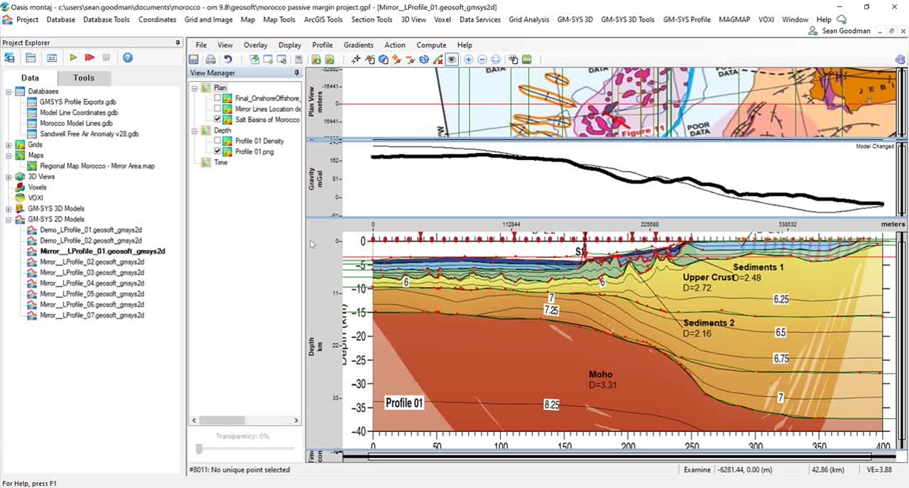
[00:16:40.210]things are slightly different in 9.8. now in GM-SYS.

[00:16:43.550]We’ve got a view manager on the left-hand side,

[00:16:45.600]and this is where we essentially manage our overlays

[00:16:48.730]within the Time, Depth and Plan windows.

[00:16:51.800]So we’ve got our Plan View window here,

[00:16:54.160]the Depth window and the Time window if we’re using it.

[00:16:58.000]So what I’m going to do is actually load in that image now.

[00:17:02.320]So Overlay, Grids and Images,

[00:17:04.390]and I can either Display a Section Grid,

[00:17:07.890]which could be at seismic line that I’ve imported

[00:17:10.790]through the SEG-Y Importer, but in this case,

[00:17:13.380]I’m going to Display an Image.

[00:17:14.540]So it can be a PNG, a BIP map

[00:17:17.551]in the old versions of GM-SYS used to load.

[00:17:24.800]So this brings up this dialog box.

[00:17:26.970]So we can go and select our image.

[00:17:28.990]So the one that I just georeferenced is Profile 01

[00:17:32.460]and it gives us the Orientation

[00:17:34.730]and we can select the Target pane.

[00:17:36.890]So I know that this one’s going into my Depth Section.

[00:17:39.710]So I’ll just select that

[00:17:41.870]and that will now load in.

[00:17:44.660]And one of the great things about 9.8

[00:17:46.880]is that we can now have multiple backdrops,

[00:17:49.560]in multiple windows.

[00:17:50.640]So I’m going to go and reload another image

[00:17:54.930]over the same window there.

[00:17:56.960]So profile 01, and this is a density image.

[00:18:00.040]And again, I’m just going to put it

[00:18:01.610]in the Depth Section there, and now that’s loaded in.

[00:18:04.770]But what happens in the View Manager

[00:18:06.770]on the left-hand side here is that they both,

[00:18:08.630]you can toggle with them on and off,

[00:18:09.840]in the same way that you can toggle surfaces

[00:18:12.480]and grids on in maps.

[00:18:15.430]So this now allows us

[00:18:19.160]to essentially go through and QC our models

[00:18:21.580]with other data and other schematic images

[00:18:26.749]and QC the models that we’ve created.

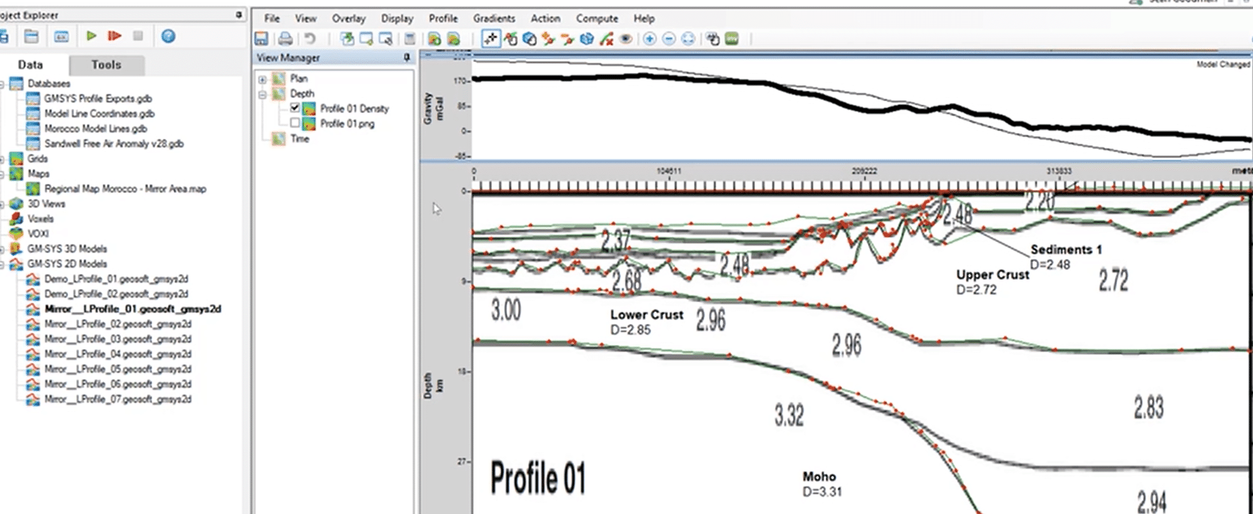
[00:18:28.910]So in this one,

[00:18:29.820]in Profile 01, we’ve got a velocity section,

[00:18:33.330]just to show velocity with depth throughout the line.

[00:18:36.760]And then, the second image really just looks

[00:18:39.230]at how density varies with depth.

[00:18:41.380]But also what we can see here is that this actually shows

[00:18:44.480]that there’s lateral variation of density.

[00:18:46.710]And so we can then incorporate that

[00:18:48.510]into different iterations of our modeling process.

[00:18:54.760]So now that we’ve got our images loaded in,

[00:18:57.170]I guess then the next thing I’d like

[00:18:58.500]to cover off is working with views.

[00:19:01.680]And the reason that working with views is important is that

[00:19:05.820]when we start to make changes to our models

[00:19:08.330]and zoom into specific areas within our model,

[00:19:11.950]it makes them much easier to come back to a single point,

[00:19:15.120]a single starting point,

[00:19:17.970]and rather than messing about with zooming in and out,

[00:19:20.470]actually just having these preset views that you’ve created

[00:19:23.960]at the start of your modeling process,

[00:19:25.700]makes things much, much easier throughout.

[00:19:28.720]So in terms of this, I’ve got in this one,

[00:19:31.420]I’ve got my Depth window,

[00:19:33.310]my Gravity, Magnetics and Plan view.

[00:19:35.830]So what I can do,

[00:19:36.663]if I want to create this as a view essentially,

[00:19:39.760]now I can go to View,

[00:19:43.630]Manage Views and I can Add Current View

[00:19:47.330]and I’ll just call it Depth Grav Meg,

[00:19:52.930]and I can add that in and press OK.

[00:19:56.330]So now when I zoom into a specific area

[00:19:59.480]to try and make some variations to surfaces,

[00:20:03.040]rather than having to zoom back out again,

[00:20:05.420]and then re-zoom in, which can take a bit of time,

[00:20:10.720]I can actually just select my view

[00:20:12.860]and it will take me back to the original point.

[00:20:15.410]And so, what I can do actually is,

[00:20:17.500]if I don’t want to look at my Plan View window

[00:20:19.860]and just have my gravity and depth window,

[00:20:22.490]I can now add that as a current view.

[00:20:25.571]And that started that in as new view, number 6,

[00:20:28.300]I can then go in and manage those views and rename that.

[00:20:32.970]So this is just makes things easier for us,

[00:20:36.030]especially when I come back

[00:20:37.320]to showing you exporting these models as images and PDFs

[00:20:41.300]at the end of the webinar.

[00:20:43.430]It shows why it’s important to really just come back

[00:20:46.330]to a single view so that you can have consistency

[00:20:49.640]across your models throughout.

[00:20:51.950]So for the next session of this webinar,

[00:20:53.850]what I’m going to do is just jump out of this model,

[00:20:55.710]and into another one.

[00:21:02.513]And I’m going to focus in this section more

[00:21:04.410]on the modeling processes itself,

[00:21:05.777]and some of the various different techniques that we can use

[00:21:08.370]in terms of auto calculations,

[00:21:10.620]using various physical prompt properties, filtering,

[00:21:14.570]and why it’s important for building robust models.

[00:21:17.690]And then, I’ll look at some of the map functionality

[00:21:20.210]within the 2.75D modeling,

[00:21:23.020]and finally touch on some inversions

[00:21:25.130]before we can leave the modeling space

[00:21:27.830]and export some horizons.

[00:21:30.220]So actually what we can see on this model now

[00:21:32.420]is that there are a few mismatches

[00:21:34.670]on the Western end of the line.

[00:21:36.930]We’ve got a bit of a negative mismatch

[00:21:38.630]between the observed and calculated data.

[00:21:42.470]So this suggests that we need more mass

[00:21:44.480]in the Western end of the line

[00:21:45.780]and less mass in the Eastern end of the line.

[00:21:48.590]And when we actually compare it,

[00:21:50.480]the current model that we have

[00:21:52.360]to the density image behind it,

[00:21:55.470]we can actually see that it’s a relatively simplistic model

[00:21:58.890]in comparison to some of the natural density variation

[00:22:01.620]that we see in the image.

[00:22:03.760]So one way that we can actually start testing scenarios,

[00:22:07.320]we can just come in and important new surface and depth.

[00:22:10.620]So we can select it in the Depth of the Time window,

[00:22:13.110]and we’d just go into Append.

[00:22:14.760]And one of the things that I’m going to focus on here,

[00:22:18.070]actually is increasing this density here.

[00:22:20.210]So at the moment we have 2.85

[00:22:22.690]for the whole of the Lower Crust,

[00:22:24.610]but clearly we varied between three grams per CC,

[00:22:30.030]all the way down to 2.83.

[00:22:32.230]It really depends in terms of where we are

[00:22:34.790]in the transition zone,

[00:22:35.970]and it seems unrealistic that we would necessarily have

[00:22:38.740]just 2.85 for the whole unit.

[00:22:41.180]So I’ll split this and increase that density there.

[00:22:50.722]And what we can then do is go into this layer here,

[00:22:56.740]this new Lower Crust, and we can actually,

[00:23:01.630]we can increase the density to see what effect that has

[00:23:05.970]on the model profile here.

[00:23:07.790]So a really nice way of doing that

[00:23:09.340]at the moment where we’ve got a 2.85.

[00:23:11.370]And, actually if we click this button here,

[00:23:14.330]we can now set a range of densities

[00:23:16.770]in which we want to test.

[00:23:19.040]So I’m going to set the limit at 2.75, and Hi of 3,

[00:23:28.290]and you can vary the linear increments as well.

[00:23:31.070]So I’m just going to leave that in 0.1.

[00:23:33.670]And now what we can actually do is

[00:23:34.990]scroll along this scroll bar here,

[00:23:38.840]and we can see what effect that has on the profile

[00:23:41.950]in real time.

[00:23:44.320]So we to land on 2.94 as the model suggests,

[00:23:49.720]and then we can Accept that and press, OK.

[00:23:53.120]We can also do that with the Magnetic.

[00:23:55.470]So Susceptibility, as well as Remnants as well.

[00:23:57.680]So where you see a A/C this means Auto Calculate.

[00:24:02.420]And so, we can run those auto calculation,

[00:24:04.810]scroll bars on all of those sections.

[00:24:08.460]So I’m just going to press OK and accept those changes.

[00:24:14.100]And one of the really important things

[00:24:15.980]about building a robust profile model

[00:24:19.270]is that we really need to start filtering the data

[00:24:22.600]to understand where and which,

[00:24:24.800]what depth our anomaly mismatches relate to.

[00:24:29.210]So, one thing we can do actually is

[00:24:30.950]by just filtering this profile in here.

[00:24:34.330]So I can run maybe just a low-pass filter.

[00:24:37.400]There are a selection of other ones,

[00:24:39.430]so I’m just going to run a low pass filter of 150,000.

[00:24:45.750]And now I can turn those filtered profiles on.

[00:24:57.136]And now this, what this does,

[00:24:59.152]it shows me-

[00:25:00.843]It’s regional filter,

[00:25:03.370]which will allow me to look at the longer wavelengths

[00:25:06.000]and what might be going on with the Moho

[00:25:07.921]and that lower crustal scale, that deeper structure,

[00:25:13.670]and that can help us guide and understand what’s going on

[00:25:17.040]in terms of the transition zone.

[00:25:19.530]So that’s really important that you actually achieve a match

[00:25:22.190]at both the long wavelengths that we have here.

[00:25:25.360]And once we start filtering with the shorter wavelengths,

[00:25:28.640]actually varying those shallow structures

[00:25:30.690]to ensure that we have a good correlation

[00:25:33.730]between our observed

[00:25:34.630]and calculated data at the longer wavelengths,

[00:25:38.350]as well as the shorter wavelengths.

[00:25:41.280]So if I just turn it back to the unfiltered version,

[00:25:45.980]then I can actually start to think about

[00:25:50.590]what the sort of form of that transition zone is there.

[00:25:55.740]So we’ve obviously got an increasing density

[00:25:58.460]as we move further seaward,

[00:26:01.380]until we get to oceanic crust,

[00:26:02.960]but whereabouts is the continental oceanic boundary?

[00:26:07.480]You don’t really know that at the moment.

[00:26:10.170]We can see a gradual transition,

[00:26:11.860]but actually one of the key things

[00:26:13.460]that we’d be looking to ascertain

[00:26:15.320]from this modeling process is where the OCB is

[00:26:19.060]or what the form and structure of the OCT is?

[00:26:22.770]If it’s more a transition zone rather than a hard boundary.

[00:26:26.020]So one thing that we can actually do is look

[00:26:28.020]at the horizontal gradient

[00:26:30.570]and what we do have here is we have the horizontal gradient

[00:26:35.830]within this, and I’ve got a view just saved already.

[00:26:38.320]So Grav-Plan View,

[00:26:41.470]and what we can see is that we’ve got a pretty strong kick

[00:26:44.530]in the horizontal gradient around here,

[00:26:46.130]which kind of lines up

[00:26:48.039]with where we’re at on the transition zone

[00:26:51.720]from continental to oceanic crust.

[00:26:55.120]I guess the benefit

[00:26:56.457]of being able to have these grids,

[00:26:58.580]such as the horizontal gradient

[00:26:59.750]within the GM-SYS planned view window now.

[00:27:01.920]It means that we don’t have to keep switching

[00:27:04.470]between the map and the model in order to be able

[00:27:07.630]to make these correlations between the maps

[00:27:10.700]and what’s going on at depth in our sections.

[00:27:14.530]So I guess some of the questions

[00:27:16.480]that you can start asking yourself,

[00:27:17.670]based on this is, is it a very prominent anomaly?

[00:27:21.520]The horizontal gradient anomaly there,

[00:27:24.250]or is it more protracted series of low amplitude anomalies

[00:27:27.570]across further distance?

[00:27:31.260]So this might help us to understand what the nature

[00:27:34.810]of the transition zone is,

[00:27:37.400]and whether it’s basically a hard boundary

[00:27:40.070]from continental to oceanic crust

[00:27:42.110]or is there a bit of a transition zone

[00:27:46.110]as we gradually increased density towards there

[00:27:48.450]or perhaps there could be,

[00:27:50.030]if we start looking at our velocity profile,

[00:27:53.060]there could be some high velocity,

[00:27:55.270]high density under plating or something like that.

[00:27:57.490]So this really, by combining these multiple section images

[00:28:01.610]and the grids in the Plan View window,

[00:28:04.100]then what we’re able to do

[00:28:05.310]is actually guide our interpretations

[00:28:07.520]and come up with a series of different scenarios

[00:28:10.770]that we can test essentially to gain some understanding

[00:28:15.020]of what’s going on within the crust at depth.

[00:28:19.050]Now, where we’ve kind of focused so far on looking

[00:28:21.390]at the longer wavelength residual errors in the profiles,

[00:28:24.810]so here and here,

[00:28:27.680]what we can actually do is also use high-pass filtering

[00:28:31.010]to understand what’s perhaps going on

[00:28:33.320]in the shallower sections

[00:28:34.580]and therefore analyze some of these shorter wavelength,

[00:28:38.990]higher frequency anomalies

[00:28:41.820]that might be due to features within the shallower section.

[00:28:46.630]So what I’m going to do is I’m going to focus

[00:28:48.370]on this particular anomaly.

[00:28:50.620]As we can see,

[00:28:51.453]it starts to look more high frequency

[00:28:54.231]compared to the anomalies

[00:28:56.450]and the mismatches at either end of the line.

[00:28:59.180]And so, what I’m wondering is that perhaps this mismatch

[00:29:03.380]could be associated with something that’s going on shallower

[00:29:06.560]in the section.

[00:29:07.890]So rather than essentially a regional low-pass filter,

[00:29:11.410]I’m actually going to change it to a high pass filter now.

[00:29:13.990]So I was on low passed before,

[00:29:16.530]so I’m just going to switch over to High pass

[00:29:19.090]and now take the Observed gravity off

[00:29:23.370]and input the filtered data.

[00:29:28.250]And what we can see is

[00:29:29.250]that we do have quite a distinct gravity low

[00:29:34.180]just in this region here.

[00:29:36.440]It does seem to coincide

[00:29:38.130]with the fact that it’s on transition zone,

[00:29:40.890]and we do have a fair bit of structure here

[00:29:43.561]in the shallower section there.

[00:29:46.520]So my thoughts are that perhaps there’s something going on

[00:29:49.880]in the shallower section of the model

[00:29:52.330]that we aren’t taking account of currently.

[00:29:54.890]And this,

[00:29:55.723]given that it’s a 400 kilometer regional scale line,

[00:29:58.700]it is quite a simplistic view of the geology.

[00:30:01.890]So when you start to high-pass filter,

[00:30:04.470]you will start to see some errors creep in.

[00:30:07.510]Now, what we actually have the benefit of is

[00:30:11.120]with our Plan View window,

[00:30:12.800]we can bring in these different maps.

[00:30:14.900]And so, we can actually correlate

[00:30:16.300]and see whether there’s anything on

[00:30:18.380]in our known geology

[00:30:19.910]that we can relate back to that anomaly.

[00:30:22.630]So I know that this is a region of salt basins.

[00:30:26.364]It’s widely documented.

[00:30:28.800]So I’ve got a georeferenced salt basins map,

[00:30:33.110]and actually this shows the the location of the line going

[00:30:36.170]through the map.

[00:30:37.003]And, actually what we can see here is that over this area,

[00:30:39.780]we do have a salt basin in here

[00:30:42.920]and these are individual salt domes that have been mapped.

[00:30:46.990]And so, what this might be telling us

[00:30:48.870]is that this particular low,

[00:30:52.110]and therefore this mismatch might be associated

[00:30:54.900]with the fact that we don’t have any salt within this model.

[00:30:58.480]So at the moment we just have 2.72 for Upper Crust,

[00:31:02.120]and then we jump into sediments of 2.48, 2.35 and then 2.2.

[00:31:08.120]So we have quite a lot of,

[00:31:11.553]there’s certainly room for error in this model,

[00:31:14.470]given that we don’t have any of this widely known salt

[00:31:18.800]that’s reflected in the model.

[00:31:21.480]So that again, that shows the power

[00:31:23.190]of being able to bring in your maps

[00:31:26.690]and your grids into this Plan View window,

[00:31:29.030]and just ensure that you are integrating all of your data

[00:31:33.010]into your modeling process.

[00:31:37.590]So not only can we incorporate our map and grid imagery

[00:31:40.960]in the Plan View window,

[00:31:42.450]to help guide our interpretation and understand the depth

[00:31:46.940]at which our anomaly mismatches really are sourced from,

[00:31:52.780]we can actually also use it to guide our 2.75D modeling.

[00:31:57.630]So the assumption in profile modeling

[00:31:59.210]is that all blocks extend to infinity along strike

[00:32:02.030]in the Y orientation.

[00:32:03.110]So in and out of the page,

[00:32:05.160]and in this instance,

[00:32:06.770]if we’re talking about a localized body such salt,

[00:32:09.430]it might be geologically unrealistic.

[00:32:11.970]So by integrating that known geological information

[00:32:14.610]from our maps and grids,

[00:32:16.070]it can help us to define how far our localized body extends

[00:32:19.600]in the Y orientation away from the profile line.

[00:32:23.300]And, therefore this helps us

[00:32:24.760]to create a more geologically feasible and robust model.

[00:32:28.440]So, in this example,

[00:32:29.910]what I’ll do is I’ll just-

[00:32:31.470]In order to create a localized 2.5D body,

[00:32:36.140]I’ve just selected this one here,

[00:32:37.570]which correlates with the anomaly low.

[00:32:41.000]And what I can now do is just click this box.

[00:32:43.130]It says 2.75D and this creates two blocks.

[00:32:47.380]So a Y positive and a Y negative block.

[00:32:51.280]And what we can do is we can come in here

[00:32:52.800]and define the length of this block.

[00:32:55.740]So I’m going to call it, let’s say 10,000 meters.

[00:33:04.083]So it’s positive and negative.

[00:33:08.537]So you input that for both and press OK to that.

[00:33:14.080]And what this now actually does, if we change our plan,

[00:33:17.590]new depth to essentially cut through this body now,

[00:33:21.750]what we can actually see is that this body here

[00:33:27.520]and this body here both have 2.75D limits.

[00:33:31.580]So we can actually go in

[00:33:32.900]and change that based on what we can see

[00:33:35.960]within those maps there,

[00:33:39.054]and that will change the nature

[00:33:42.590]of that anomaly there as well.

[00:33:45.320]And so, we can see how that varies,

[00:33:47.430]if we move that Plan View again,

[00:33:48.850]then we actually see more of the body there.

[00:33:52.980]And so, in this example, it’s obviously more regional scale.

[00:33:56.238]So we’re not going to be looking at individual salt bodies,

[00:33:58.900]but if we had a more focused

[00:34:00.920]and more localized body that we wanted to analyze

[00:34:03.990]and model in 2.75D,

[00:34:06.350]then this incorporation

[00:34:07.760]of the map functionality really helps us to do that

[00:34:10.180]in a more accurate way.

[00:34:12.700]So what I’ve shown you so far has really been

[00:34:14.590]around the concept of forward modeling.

[00:34:16.410]So that’s changed where the interpreter

[00:34:18.760]really makes alterations to the model geometries

[00:34:21.160]and physical properties to attain a fit

[00:34:23.620]between the observed and calculated anomaly data.

[00:34:26.490]Now, what we can also do is run a 2D inversion

[00:34:29.100]which allows us to define certain points and parameters,

[00:34:33.260]which GM-SYS will then alter

[00:34:35.050]to achieve a correlation between the observed

[00:34:37.170]and calculated profiles.

[00:34:39.250]So I’m just going to remove this filtered data now,

[00:34:42.630]and I’m going to replace it

[00:34:43.630]with the original, observed data.

[00:34:49.020]So now, what we can do

[00:34:49.920]is actually just run a quick 2D inversion

[00:34:51.950]on some various aspects of these models.

[00:34:54.230]So it might be varying individual points,

[00:34:57.220]in terms of structure,

[00:34:58.200]or we might vary the Susceptibility or Density

[00:35:02.710]within some of these layers.

[00:35:04.820]So I’m going to come to Action and Invert.

[00:35:09.845]And so, what this now allows us to do

[00:35:11.050]is select what type of inversion we’re going to run.

[00:35:13.300]So in this respect, I’m going to change Density.

[00:35:17.060]And then, in density and susceptibility and inversions,

[00:35:20.210]You click on a specific layer.

[00:35:21.900]So here I’m going to select that salt body

[00:35:24.150]that we just looked at.

[00:35:27.050]So we’re going to keep auto DC Level ticked,

[00:35:29.320]and we can add in some constraints if we want to.

[00:35:32.330]So if we select this box and then click Constraints,

[00:35:35.010]we can essentially define a maximum change in X and Z.

[00:35:40.390]If we’re invert on those,

[00:35:43.080]and we can also change the gravity ratio,

[00:35:45.360]if we’re doing a combined gravity and magnetic conversion.

[00:35:48.170]So for this one,

[00:35:49.250]I’m just going to press GO and see what happens.

[00:35:51.570]So as you can see, we’ve had a bit of a change there.

[00:35:54.150]The dashed line shows where the old calculated profile was,

[00:35:58.770]and this is now the new form based

[00:36:01.130]on that inversion results.

[00:36:02.210]So we can see a change in gravity here of 1.839.

[00:36:07.090]And so, we can keep doing a number of steps here just

[00:36:10.440]to see what fit we get.

[00:36:12.600]In this one,

[00:36:13.433]it’s not going anywhere cause it’s been pushed

[00:36:14.950]as far as it can go.

[00:36:18.350]So I’m going to undo those,

[00:36:20.660]but I’m going to select Accept on this one.

[00:36:25.120]And now, what I can do is actually

[00:36:26.610]just quickly move the label

[00:36:30.210]Each time you run an inversion,

[00:36:32.610]it will update this density value in the labels there.

[00:36:35.200]So what I can see is that isn’t a realistic value there.

[00:36:39.810]So I’m going to change that back

[00:36:44.910]to 2.16, and now, again, this is back to being where it was,

[00:36:51.870]but that shows that-

[00:36:55.110]So what that shows is really two things.

[00:36:57.490]Actually, I can run multiple iterations of an inversion

[00:37:00.125]to get to a point at which I’m happy with the density

[00:37:04.100]or susceptibility or the result of the inversion,

[00:37:07.290]but it also shows the importance

[00:37:09.120]of not just letting the program run

[00:37:12.570]with the inversion by itself,

[00:37:13.670]but actually QCing the inversion

[00:37:15.360]because what it might do is create something

[00:37:18.100]that’s not geologically feasible.

[00:37:20.160]So whilst it’s good

[00:37:21.730]for testing different scenarios quite quickly,

[00:37:25.320]you’d certainly do need

[00:37:26.420]to make sure that your QCing what it produces there as well.

[00:37:30.670]So for the next step of the inversion workflow,

[00:37:34.420]I’m going to look at varying the points themselves.

[00:37:38.680]So what we can do is we’re able

[00:37:40.320]to select a number of points.

[00:37:41.890]So in this example,

[00:37:42.880]I’ll focus in this section of the model

[00:37:45.300]and what we can do is select a number of points,

[00:37:47.730]which we will allow the inversion to move for us.

[00:37:51.500]And the remaining points would essentially be locked

[00:37:53.540]in their current positions.

[00:37:54.560]So we can add in extra points.

[00:37:56.310]We can remove points prior to inversion

[00:37:58.830]and that’s going to help us decide

[00:38:01.160]on the level of detail that we require.

[00:38:03.470]So, if it’s a very regional scale inversion,

[00:38:05.660]we might have very few points.

[00:38:07.370]But if we need quite complex geometries

[00:38:10.300]to be taken into account,

[00:38:12.070]then we might be able to add in some extra points

[00:38:15.330]and then select those points to then be moved

[00:38:18.490]or free or fixed in the inversion.

[00:38:22.500]So, if you’ve got a more targeted area

[00:38:24.290]that you need to model,

[00:38:25.520]this model can actually, in fact,

[00:38:27.360]be much faster than manually editing those individual points

[00:38:30.510]in a forward modeling workflow.

[00:38:32.860]So I’m just going to jump back into that invert.

[00:38:36.260]So here, we’ve got Free/ Fix in Z.

[00:38:41.640]I’m going to keep also Auto DC Level is ticked,

[00:38:44.910]and my Constraints,

[00:38:45.760]I’m going to allow maximum of 2 km movement

[00:38:49.267]in the Z orientation.

[00:38:50.750]So now, we can go through and select the points

[00:38:52.720]that I want to be free.

[00:38:54.390]So these can move during the inversion process.

[00:38:59.190]And then, I’m just going to press GO

[00:39:00.720]and see how this changes.

[00:39:03.060]So we can see that obviously,

[00:39:04.760]with the negative mismatch that we’ve gotten the calculated

[00:39:07.820]and observed data,

[00:39:09.100]is trying to increase or shallow this horizon here.

[00:39:14.290]So I’m going to press Next Step

[00:39:16.220]and this will just keep making changes

[00:39:18.200]to the inversion until

[00:39:20.622]to the surface, until such a point that we get a better fit.

[00:39:27.230]So what I could actually now do is press Accept on this.

[00:39:30.740]I could clear all of those points,

[00:39:33.250]and I could change just this point and this point,

[00:39:36.940]and I could actually add an a point as well,

[00:39:40.610]to add in some more detail to the inversion.

[00:39:46.860]And I can press GO again on that.

[00:39:49.130]So that can then localize that.

[00:39:50.950]And whilst that’s perhaps not a very realistic,

[00:39:53.960]we’d probably actually have more of a combination

[00:39:56.470]of varying the surfaces, as well as the density

[00:40:00.730]within that layer as well.

[00:40:02.460]So I’m going to just quickly undo all of those,

[00:40:08.860]and just press Clear All

[00:40:10.010]and that removes all of those free points

[00:40:14.670]and I’m just going to come out of that now.

[00:40:16.140]So I’m actually going to move those points back,

[00:40:19.760]so I can select a group of points.

[00:40:22.000]So mark points in a box

[00:40:24.237]and I can select all of those points

[00:40:27.860]and drag those back down to where they were,

[00:40:30.670]prior to the inversion.

[00:40:33.180]So I’ll just clear those now.

[00:40:35.670]So that’s everything

[00:40:36.503]in terms of just running through the features

[00:40:39.680]that can assist you in your interpretation workflow.

[00:40:44.000]And now, what I’m going to go back

[00:40:45.430]and focus on is just getting to that export stage

[00:40:48.160]in terms of exporting models, as images and PDFs,

[00:40:50.860]if you want to put them into a report

[00:40:52.760]or as if you need to export horizons,

[00:40:55.490]which you want to grid up

[00:40:56.530]and put into other interpretation packages as well.

[00:41:00.470]So I’m going to quickly save this model.

[00:41:04.910]And this really, when you start to get to this stage,

[00:41:08.520]we’re talking about the importance of views again.

[00:41:11.130]So, obviously, we’re working on the Gravity,

[00:41:13.860]Plan View and Depth windows,

[00:41:15.410]but if I wanted to, say export something

[00:41:18.440]that’s just the Gravity and the Magnetic window,

[00:41:20.520]or one of my previously saved views,

[00:41:23.790]I can then go back to Gravity and Depth.

[00:41:26.340]And this will take me back

[00:41:27.410]to that specific view that I would like to export as well.

[00:41:32.090]So if we get to a point where we’ve got an image

[00:41:34.510]that we’re happy with,

[00:41:36.020]we can go to the print button

[00:41:39.130]and this will open up the page layout menu.

[00:41:44.170]And so we can either print to PDF,

[00:41:47.500]or we can do Raster Drive for GM-SYS.

[00:41:49.950]This will allow us to create a PNG, BIP map,

[00:41:53.280]any other image file.

[00:41:57.440]And then we can go into-

[00:41:59.500]You can obviously set up your printer,

[00:42:01.170]but we can set up the page layout.

[00:42:03.180]So in this example, we’ve got sort of the time window

[00:42:05.610]at the bottom, Depth window, Gravity, Magnetic

[00:42:08.810]and Plan View,

[00:42:09.920]and we’ve got various title boxes around the edge.

[00:42:12.760]So I’ve been working in the depth window this whole time.

[00:42:15.440]So actually when it comes to printing or exporting images,

[00:42:18.960]I don’t need this time window.

[00:42:20.540]So what I can do is go into my page setup layout,

[00:42:25.080]and I can go to Time and just put 0 in there

[00:42:28.380]and that will remove that pane from there now.

[00:42:31.720]You can then go through and very the aspect ratio.

[00:42:34.590]You can vary the sizes of all your windows.

[00:42:39.120]You can vary the layout, in terms of the margins,

[00:42:42.810]so the top and left margins.

[00:42:45.730]So, if I wanted to increase the size of my Depth windows,

[00:42:48.750]so I know it goes down to 40 km,

[00:42:51.410]and I can increase my vertical saturation,

[00:42:54.160]Let’s say to 6,

[00:42:55.120]to make that a much larger window on the page.

[00:43:00.120]I can do the same for the Gravity and Magnetic windows.

[00:43:04.720]So at 1.5 inches.

[00:43:11.050]And I might want to keep my Plan View windows

[00:43:12.910]smaller than those.

[00:43:13.830]So if I want to keep it as 1 inch,

[00:43:15.610]then that’s fine.

[00:43:16.443]So I can then press OK on that.

[00:43:17.900]And that’s my page set up for export.

[00:43:21.210]So, what I can then do,

[00:43:22.420]and if I want to keep that page set up exactly the same,

[00:43:27.420]if I have to produce a series of these images

[00:43:30.050]for reports or publication,

[00:43:32.500]what I can actually do is save that config here.

[00:43:37.140]And so, I can just save it within the project directory

[00:43:40.880]and any other time,

[00:43:42.180]when I come back in here,

[00:43:43.220]I can just, again, load it in from there.

[00:43:46.140]And then once I press Print,

[00:43:47.690]that would allow me to export as PNGs, BIP maps, GeoTIFFs,

[00:43:52.110]any of those images as well.

[00:43:55.270]And the final aspect of today’s talk really is going

[00:43:59.090]to come back to exporting horizons in an efficient way.

[00:44:03.490]So this really,

[00:44:04.770]it jumps back into the importance of managing our horizons

[00:44:08.550]and blocks efficiently,

[00:44:10.190]at the start of the modeling process,

[00:44:11.970]which now once we get to this point of export,

[00:44:14.770]it makes our lives a lot easier.

[00:44:16.950]So what I can do is go to GM-SYS Profile.

[00:44:19.910]I can select my active models.

[00:44:21.900]So in this, I’m going to go with these seven models.

[00:44:25.860]So these are my project models.

[00:44:27.570]I’m going to add these to the active models list,

[00:44:31.310]and that will now validate them,

[00:44:33.600]and understand which horizons are in which models,

[00:44:36.250]in which blocks there are as well.

[00:44:39.050]And then once we’ve exported those,

[00:44:40.340]we can jump into GM-SYS Profile,

[00:44:41.950]and go to Extract Horizons to Database.

[00:44:45.440]And so, this will now create us a horizon list

[00:44:47.960]based on the horizons that are active in each of our models.

[00:44:51.780]And, because we’ve got a seven models,

[00:44:53.410]that can take a little bit of time.

[00:44:56.810]And so, what we can now do,

[00:44:58.394]we can have a look at what horizons we have

[00:45:00.490]within our list there.

[00:45:03.370]We can select our output database name.

[00:45:05.250]So I’m just going to call it Demo

[00:45:07.860]and we can decide where our sampling location is,

[00:45:12.050]so it can be modeled profiles.

[00:45:13.870]So each of these points along the line.

[00:45:17.240]We can call it the Gravity Stations

[00:45:19.450]or the Magnetic Stations.

[00:45:20.700]So in this example, it’s 300 meters

[00:45:22.770]from the database that we originally made them from.

[00:45:30.320]And we can also look at the sample interval

[00:45:32.620]if we want specify a specific sampling tool.

[00:45:35.650]So in this example,

[00:45:36.720]I’m just going to export the Moho and the Lower Crust

[00:45:39.400]and add that to what I already have in there

[00:45:41.130]for the Upper Crust.

[00:45:42.820]And then I can just press, OK.

[00:45:46.830]And this will now generate the new horizons database

[00:45:50.190]for those seven lines.

[00:45:56.261]And again, it just takes a little bit of time

[00:45:57.930]’cause there’s seven lines to extract from

[00:46:00.210]and now this is the the database that it’s just exported.

[00:46:06.380]So as we can see, we’ve got the seven lines in here,

[00:46:10.581]all named based on the models.

[00:46:12.100]We’ve got the X, the Y,

[00:46:13.430]and then all of our horizons that we exported as well.

[00:46:17.180]And so, now what we can actually do

[00:46:18.510]is we can look to extract these

[00:46:20.860]if we need it in a text file or anything like that.

[00:46:22.740]So we can go to Database Export, Geosoft X, Y, Z

[00:46:26.540]and just name it, whatever we need to name it.

[00:46:29.080]We can also grid up each

[00:46:30.620]of those horizons via minimum curvature,

[00:46:33.950]and then once we have those in a grid,

[00:46:35.700]we can export those to any file format that we need to,

[00:46:38.590]such as Landmarks Z-map,

[00:46:40.460]which might allow you to put it

[00:46:41.810]into another interpretation package.

[00:46:45.260]So that’s everything we’re going to cover off today.

[00:46:47.180]We’ve covered off quite a lot in the last 50 minutes.

[00:46:49.430]So we’ve looked at the different methods

[00:46:51.550]for building profile models,

[00:46:53.250]the importance of working with views

[00:46:55.040]and managing your horizons

[00:46:57.110]and blocks across multiple models,

[00:46:59.750]and how that can really help you

[00:47:01.010]when it comes into exporting models

[00:47:03.030]at the end of your interpretation process.

[00:47:06.340]We’ve looked at auto calculations,

[00:47:08.250]inversions, the new functionality in 9.8,

[00:47:11.560]in terms of incorporating map functionality

[00:47:14.220]to aid your 2.75D modeling.

[00:47:16.650]And we’ve also looked at the importance of filtering

[00:47:19.850]throughout the modeling process as well.

[00:47:22.700]Now, just before we finish up today’s webinar,

[00:47:24.650]I just wanted to mention the variety

[00:47:26.520]of learning enrichment resources that we’ve been developing

[00:47:29.050]over the last few months.

[00:47:31.020]You can find out a bit more information

[00:47:32.900]about Oasis montaj and GM-SYS on these two solution pages

[00:47:37.180]and learn a bit more about how they can help you reduce risk

[00:47:40.060]and uncertainty in your workflows.

[00:47:42.770]We also have a variety of virtual training events

[00:47:45.180]that you can participate in,

[00:47:46.590]as well as self-serve learning pathways,

[00:47:49.290]which can be accessed in myseequent, Seequent IDs.

[00:47:54.200]You’ll also find the self-serve store

[00:47:55.810]where you can purchase Leapfrog and VOXI products.

[00:47:58.450]And for any support related queries,

[00:48:00.170]you can either get in touch with our great support team

[00:48:02.550]or head to the, myseequent support page,

[00:48:05.030]which holds over 5,000 knowledge base articles

[00:48:07.590]to help you with your everyday Oasis montaj workflows.

[00:48:11.720]So that’s all for today, everyone.

[00:48:13.040]And I’d like to thank you all for taking the time to tune in

[00:48:15.680]and hear more about our updates and workflows.

[00:48:18.280]So have a great day.