Leveraging Open Geoscience Data

Learn how you can do a desktop study using Oasis montaj, DAP and Geoscience Data Portals, incorporating various types of data to improve the planning on your early-stage exploration projects.

Overview

Video Transcript

[00:00:06.440]<v ->Hello everyone and welcome to today’s webinar,</v>

[00:00:09.010]Leveraging Open Source Geoscience.

[00:00:11.860]My name is Geoff Plastow

[00:00:13.220]and I will be your online host today.

[00:00:15.970]I am a senior geophysicist at Seequent,

[00:00:17.960]and I’m currently based in Vancouver, Canada.

[00:00:21.400]Before we get started, I would like to go over a few items

[00:00:23.880]so you know how to participate in today’s event.

[00:00:27.280]During the webinar, you will have the opportunity

[00:00:29.180]to submit text questions

[00:00:30.530]by typing your questions into the chat pane

[00:00:32.810]of the go-to webinar control panel.

[00:00:35.460]You can send in your questions

[00:00:36.510]at any time during the presentation.

[00:00:38.630]If we are unable

[00:00:39.670]to answer your questions during the session,

[00:00:41.490]we will respond to you via email in the next 24 to 48 hours.

[00:00:47.060]This morning I’m excited to speak to you

[00:00:48.800]about open geoscience data.

[00:00:51.650]During this webinar, I’m going to show you

[00:00:53.930]where you can download

[00:00:55.130]freely publicly available geoscience data,

[00:00:58.440]how you can import this data,

[00:01:00.320]and then a quick example of machine learning applied

[00:01:02.710]to open source geoscience data.

[00:01:05.410]First, we’re going to discuss the benefits

[00:01:07.630]of open geoscience data

[00:01:09.150]and some of the solutions we offer at Seequent.

[00:01:12.240]Next, we’re going to take a look

[00:01:13.500]at some real world examples of geoscience data portals

[00:01:16.380]that are open and available to anyone

[00:01:18.170]with a web browser and internet connection.

[00:01:21.830]We’re going to spend the majority of our time

[00:01:23.390]working in Oasis montaj,

[00:01:24.830]and I’m going to show you how you can easily search

[00:01:26.890]and download public domain data

[00:01:28.600]right from within the application.

[00:01:31.590]In the second half of the webinar,

[00:01:33.390]we’re going to have some fun.

[00:01:34.320]We’re going to take a look at the open API

[00:01:36.260]within Oasis montaj and target,

[00:01:38.310]and I’m going to show you some freely available tools

[00:01:40.540]you can use on your exploration project.

[00:01:43.370]And finally, we’re going to use

[00:01:44.463]some open source machine learning.

[00:01:46.370]Specifically, we’re going to take a look

[00:01:48.240]at self-organizing maps

[00:01:49.690]and how we can use this freely available tool

[00:01:52.320]to enhance or even accelerate

[00:01:54.290]an early stage exploration project.

[00:01:58.360]First, let’s talk about open geoscience.

[00:02:00.840]When geoscience data is readily accessible

[00:02:03.020]in a meaningful way,

[00:02:04.450]it supports broad social, economic

[00:02:06.890]and environmental challenges.

[00:02:08.790]Everything from land use, planning, water management,

[00:02:12.270]climate studies

[00:02:13.400]to environmental impact and reclamation assessments.

[00:02:17.740]Open geoscience data spurs inter-governmental

[00:02:20.860]and departmental collaboration.

[00:02:23.110]But moreover, it allows for a shift

[00:02:25.110]from often isolated research to industry partnerships

[00:02:28.580]and knowledge transfer.

[00:02:30.270]This results in innovation, sustainability,

[00:02:32.650]and a democratization of geoscience data for all.

[00:02:36.950]Easily accessible pre-competitive data

[00:02:39.290]also means that geoscientists can build on existing data

[00:02:42.680]and use it for their own research

[00:02:44.300]and develop new innovative methods and applications

[00:02:46.890]and integration into their own models.

[00:02:50.950]Currently sequence solutions are used at geological surveys

[00:02:54.130]and government agencies around the world.

[00:02:56.240]Here are just a few of these organizations.

[00:02:59.430]A common thread through all of these government agencies

[00:03:01.800]is their mandate to serve the public in an open,

[00:03:03.950]collaborative and informative way.

[00:03:06.430]Government geoscience data has ongoing value.

[00:03:09.320]Some would say that’s even a renewable resource.

[00:03:12.720]This renewable resource enables us

[00:03:14.620]to use and reuse geoscience data for many years to come

[00:03:18.580]and to stimulate new exploration.

[00:03:21.530]With the need for industry to explore deeper

[00:03:24.090]and undercover,

[00:03:25.160]pre-competitive geoscience data becomes even more valuable.

[00:03:28.930]And we know that applying the geological knowledge

[00:03:31.260]of known deposits and regional data sets,

[00:03:33.950]we can increase the chances of finding more deposits

[00:03:36.740]through predictive analysis, data fusion,

[00:03:39.610]and machine learning.

[00:03:41.240]If we turn our attention to the mining industry

[00:03:43.300]and resource exploration,

[00:03:44.940]on an industry-wide basis,

[00:03:46.390]this is a relatively high risk activity

[00:03:48.760]with an average timeline to discovery of 10 to 20 years

[00:03:53.110]and often two to three companies exploring a property

[00:03:56.100]before a major discovery is found.

[00:03:59.250]Due science data that is collected

[00:04:01.370]and curated by governments provide the foundation

[00:04:04.300]for early stage exploration.

[00:04:07.020]Studies have shown that investing just $1 in the acquisition

[00:04:10.400]and curation of open geoscience data

[00:04:12.920]can stimulate anywhere from 3 to 20 times

[00:04:15.780]the investment in exploration

[00:04:17.450]and considerably more if a discovery is found.

[00:04:21.410]We know that pre-competitive data stimulates, innovates

[00:04:25.010]a collaboration in our industry.

[00:04:27.430]Seequent has several data management solutions depending on

[00:04:30.630]the size, scope and objective of your geoscience project.

[00:04:34.570]These include Seequent Central

[00:04:35.910]which allows geoscientists to collaborate on earth models,

[00:04:39.740]there’s also MX Deposit

[00:04:40.770]which offers secure cloud hosted drill hole

[00:04:43.130]and sample data management.

[00:04:44.890]Two solutions that we’re going to take a look at now

[00:04:47.320]are DAP and geoscience data portals.

[00:04:51.330]DAP and geoscience portals enable a natural experience

[00:04:54.190]to search, identify, download,

[00:04:56.790]and integrate multi-discipline geoscience data.

[00:05:00.100]Geosoft DAP is server technology for publishing

[00:05:04.170]and distributing vast quantities of exploration data.

[00:05:08.480]DAP includes native support

[00:05:10.100]for most industry standard formats

[00:05:13.420]and is well integrated into GIS platforms.

[00:05:17.880]DAP server enables exploration organizations

[00:05:20.794]and government agencies

[00:05:22.700]to catalog manage, deliver,

[00:05:25.890]visualize large volumes of geospatial data.

[00:05:30.100]By doing this, they have a robust delivery solution

[00:05:33.750]for large geoscience datasets.

[00:05:38.580]Geoscience data portals allow

[00:05:41.230]the discovery of geoscience exploration data

[00:05:44.710]in a simple web interface.

[00:05:47.800]It’s easy to use

[00:05:49.450]and it also simplifies workflows

[00:05:51.150]and minimizes the requirement of reformatting, reprojecting

[00:05:54.550]and converting data types.

[00:05:56.620]Users have the ability to create maps and annotate maps,

[00:06:00.750]and they can share them using bookmarks.

[00:06:03.760]This also supports the distribution of open geoscience data

[00:06:08.330]that can be used by a variety of exploration softwares.

[00:06:12.720]So let’s take a look at a geoscience data portal

[00:06:15.850]that’s powered by DAP server technology.

[00:06:18.960]Don’t worry, we’re going to send through

[00:06:20.040]a list of all of these URLs.

[00:06:22.670]So now I’m going to switch over to a web browser

[00:06:24.400]and then following that,

[00:06:25.310]I’m going to jump into Oasis montaj.

[00:06:27.880]So here we are.

[00:06:28.850]This is the Geosoft geoscience data portal.

[00:06:33.070]It’s absolutely free to use.

[00:06:35.200]All you need to do is sign in with your Seequent ID.

[00:06:39.030]On the left-hand side,

[00:06:40.140]we have some search options that allow us

[00:06:42.620]to define where we want to search.

[00:06:45.600]We can also search for specific items

[00:06:47.840]by typing them into our keyword search.

[00:06:50.990]So if we want, we can select a specific region in the world.

[00:06:54.910]Right away, we can select a country.

[00:06:58.000]I’ll select Canada.

[00:06:59.740]And if we want, we can draw or redraw our area

[00:07:04.050]that we want to search in.

[00:07:06.150]If we ever want to go back,

[00:07:07.180]we can just jump back to a global view.

[00:07:10.590]Once we’re happy with the area that we’ve defined,

[00:07:14.220]we can just click the Search button.

[00:07:16.080]You’ll see that the search is pretty quick

[00:07:18.530]and provides us a number of geoscience results

[00:07:23.320]that we can immediately display in our web browser.

[00:07:27.120]So the first thing I’m going to do

[00:07:28.210]is I’m just going to select some topography data.

[00:07:33.120]And you’ll see that this preview loads pretty quickly.

[00:07:37.050]And it also allows me

[00:07:39.738]to adjust some of the transparency of this layer

[00:07:44.180]in the event I need to see through

[00:07:45.960]some of the map layers

[00:07:47.860]and I can also load in other geoscience information.

[00:07:51.720]In this case, I’m going to look at

[00:07:53.600]a grid of the total magnetic intensity.

[00:07:57.090]So we can begin to layer and create our own maps.

[00:08:00.850]What’s great is I can create some annotations.

[00:08:04.520]So I can add some text, I can draw some points or circles.

[00:08:09.630]So I’m going to say, “This is my exploration area”,

[00:08:18.930]and I can simply begin to draw right on this map.

[00:08:23.090]I can add a circle if I want,

[00:08:25.940]I can adjust the transparency of the fill of my objects,

[00:08:31.990]and whenever I’m ready, I can click Share

[00:08:35.950]and it’s going to create an email link,

[00:08:39.320]and I can just copy and paste this or use it in an email.

[00:08:43.230]And I’m just going to open a new tab here.

[00:08:47.800]And you’ll see that this link is a shareable link.

[00:08:49.940]And I can send this to my colleagues

[00:08:53.110]and it contains all the annotations,

[00:08:56.000]and it’s just loading,

[00:08:56.833]and it contains the data that I was looking at.

[00:09:03.570]So we also have the option to download this data, right?

[00:09:07.510]So if I click this little download button,

[00:09:10.190]we have some options of whether we want to window it

[00:09:13.070]to our exploration areas.

[00:09:15.660]So that would be the area that we searched in.

[00:09:18.350]We can say do not window.

[00:09:19.470]We have some options as well as what sort of resolution

[00:09:22.730]we want to use,

[00:09:23.980]and once we’re happy, we can say Add To Download Manager.

[00:09:27.490]It automatically zips it for us on the server,

[00:09:30.650]and we can click download and it will download.

[00:09:35.310]So you can see that navigating

[00:09:36.920]and using geoscience data portals is pretty straightforward.

[00:09:40.490]We can easily customize our search areas,

[00:09:44.980]it’s very fast and responsive

[00:09:46.680]as far as previewing the data that you want to download,

[00:09:50.070]we can create quick annotations

[00:09:52.230]and share them with our colleagues,

[00:09:53.980]and once we’re ready,

[00:09:55.260]we can easily download this data

[00:09:57.150]and open it on Oasis montaj, Target,

[00:09:59.780]and now even Leapfrog Geo.

[00:10:02.130]So this concludes my quick tour of geoscience data portals.

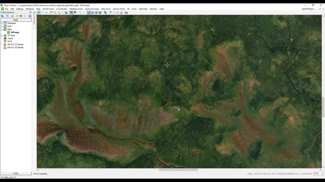
[00:10:05.880]Now let’s jump into a Oasis montaj.

[00:10:09.430]Okay.

[00:10:10.263]So now I’ve switched over to Oasis montaj.

[00:10:12.717]And I believe I mentioned this at the introduction,

[00:10:14.990]but if you’re also working in Target,

[00:10:17.160]all of the steps that I’m going through

[00:10:18.610]are exactly the same.

[00:10:20.570]The first thing I’m going to do

[00:10:21.910]is I’m just going to import a shape file.

[00:10:24.310]And this shape file is going to represent

[00:10:26.690]our area of interest.

[00:10:28.690]Perhaps this is an area that we are interested

[00:10:31.160]in doing some exploration

[00:10:32.690]or maybe it’s an area

[00:10:33.523]that we are already doing some exploration in.

[00:10:36.940]And this black rectangle here represents

[00:10:39.790]our area of interest.

[00:10:41.980]The first thing I’m going to do is go to the Seek Data menu.

[00:10:45.700]And Seek Data is going to connect us in

[00:10:48.000]to open source geoscience data.

[00:10:50.930]We have a couple of options.

[00:10:52.240]We have Seeker

[00:10:53.330]and we also can download some aerial imagery from Bing Maps.

[00:10:57.540]So I’m going to do that first.

[00:10:59.330]We have some options

[00:11:00.320]whether we want the aerial, road or hybrid.

[00:11:02.730]I’m just going to stick with Ariel for now.

[00:11:05.460]And you can see once I selected it downloads pretty quickly.

[00:11:09.510]I’m just going to click B on my keyboard

[00:11:11.720]and I’m going to select an area that we can zoom in on.

[00:11:17.060]And you can see that when I zoom in in an area,

[00:11:20.730]it redownloads or rerenders the image

[00:11:23.590]at a higher resolution.

[00:11:25.240]This is incredibly useful,

[00:11:27.330]especially for looking for areas that have cover

[00:11:29.620]or maybe we’re interested in some areas

[00:11:31.370]that have some exposure.

[00:11:33.590]Or maybe we want to see if there’s any rivers or swamps

[00:11:37.180]or roads in our exploration area.

[00:11:40.150]I’m just going to press F to zoom out

[00:11:42.350]to the extents of the map.

[00:11:46.680]Okay.

[00:11:47.660]So let’s now use the Seeker functionality

[00:11:50.150]in Oasis montaj or Target

[00:11:52.230]to connect into some DAP servers.

[00:11:55.980]I’m just going to rescale this window here.

[00:11:58.260]And what you’ll notice is right away Seeker took

[00:12:02.340]the extents of our area of interest on our map

[00:12:07.110]and has defined that as our main search criteria.

[00:12:11.720]We can move this area around,

[00:12:14.320]we can resize it if we want,

[00:12:16.560]we can jump out to a global view,

[00:12:19.420]and if we hit refresh,

[00:12:20.610]again, it will bring us back to the extents of the map.

[00:12:24.870]We have some options here

[00:12:26.500]if we want to search for something specific,

[00:12:28.490]maybe geochemistry data or existing drill hole data,

[00:12:32.370]and we also have the option to do an advanced search.

[00:12:35.270]So we can use some metadata,

[00:12:36.940]so maybe that is a specific format

[00:12:39.490]or data of a specific scale or resolution.

[00:12:42.560]We can build a relatively complex search criteria

[00:12:45.910]if we want.

[00:12:47.510]Usually when I’m just starting off,

[00:12:49.200]I’m going to go ahead and just do

[00:12:51.211]just a general search to see what is available.

[00:12:54.420]And you can see here

[00:12:55.950]we have results from two public DAP servers.

[00:12:59.520]We have our natural resource Canada DAP server

[00:13:02.400]which has given us 254 datasets

[00:13:05.800]and we also have the Geosoft DAP server.

[00:13:09.470]And both of these are two different servers.

[00:13:11.800]And it allows us to download various geoscience data.

[00:13:16.290]So let’s take a look at what’s in the typography folder

[00:13:19.650]on the Geosoft DAP server.

[00:13:21.560]So I can click on this,

[00:13:23.210]and what’s great is it will automatically give us

[00:13:26.470]a preview of the data set that we’re downloading

[00:13:30.000]so we can see what the SRTM

[00:13:31.780]or the topography data looks like.

[00:13:35.150]Now, if I jump back into the natural resource Canada website

[00:13:39.800]or DAP server,

[00:13:41.120]we can look at some of the other layers that are available.

[00:13:45.070]We have drainage and roads and NTS sheets.

[00:13:49.140]These are incredibly useful for us.

[00:13:53.169]I’m going to take a look at what’s available

[00:13:55.820]as far as geophysical data.

[00:13:58.350]We have some EM data and some magnetic data,

[00:14:02.550]and what I’m going to do

[00:14:04.010]is I’m going to download some total magnetic intensity

[00:14:09.540]from within the survey area,

[00:14:11.860]and I’m going to also download

[00:14:14.200]some late time apparent conductivity.

[00:14:17.600]This was part of an airborne electromagnetic

[00:14:20.380]and magnetic survey.

[00:14:23.600]So here, what I’m going to do now is download this data.

[00:14:27.780]These are the grids that I’m going to download.

[00:14:31.220]And when I click on them, I have some options.

[00:14:33.900]It gives me some options of where I save these two,

[00:14:36.640]whether I want to rename it,

[00:14:38.110]the type of file,

[00:14:40.220]and whether I want to display them when I download them.

[00:14:44.340]Some great options here are when we download the data,

[00:14:48.450]do we want them all in the same projected coordinate system?

[00:14:52.550]Typically, when I work with data

[00:14:53.840]I like having everything in the same coordinate system,

[00:14:58.240]so I can apply this to all of the grids that we download.

[00:15:02.530]We also have some options

[00:15:04.460]whether we want to down sample

[00:15:06.230]or keep the original resolution.

[00:15:09.278]In this case I’m just going to keep

[00:15:10.660]all of the original resolution.

[00:15:14.020]And once I click Download,

[00:15:15.920]it’s going to reach out to these two different DAP servers,

[00:15:19.300]one hosted by natural resource Canada

[00:15:21.470]and one hosted by Geosoft,

[00:15:23.460]and it’s going to download these two grids onto my computer.

[00:15:28.900]So that happened pretty quickly.

[00:15:30.410]Let’s take a look at the results.

[00:15:35.330]So now I’m just going to expand the map manager,

[00:15:37.940]and I’m going to pin this open so we can take a closer look

[00:15:41.040]at some of the map layers that we just downloaded

[00:15:43.380]from two different DAP servers.

[00:15:46.210]The first layer I’m going to look at

[00:15:47.330]is our SRTM topography data.

[00:15:50.230]And what’s great is it covers the complete project area

[00:15:53.630]and it downloaded and is geo-referenced

[00:15:56.580]into the correct location.

[00:15:58.730]I’m just going to adjust the transparency of this layer

[00:16:01.890]to give just a little bit of context to our aerial imagery.

[00:16:06.520]So now we can just correlate some of the rivers and lakes

[00:16:10.310]to areas of higher topography.

[00:16:13.750]Next, let’s take a look at some of the geophysical data

[00:16:16.620]that we downloaded.

[00:16:19.100]Again, this is a grid of the total magnetic intensity

[00:16:23.810]across the survey area.

[00:16:25.660]The areas that are red or hot in color represent areas

[00:16:28.890]of a high magnetic intensity

[00:16:30.937]and the areas that are blue or cool in color represent

[00:16:34.520]an area of a low magnetic intensity.

[00:16:38.030]And again, what’s great is all of these grids came in.

[00:16:41.520]We didn’t have to worry about coordinate conversions

[00:16:44.970]or changing of file types,

[00:16:46.570]all of that happened through the DAP server.

[00:16:51.140]Let’s take a look at the other grid that we downloaded.

[00:16:53.830]This is the EM component of the survey.

[00:16:56.300]This is the apparent conductivity.

[00:16:59.170]The areas that are pink or hot in color represent areas

[00:17:03.340]of a high apparent conductivity.

[00:17:05.890]The areas that are blue or cool represent

[00:17:08.110]an area of low apparent conductivity.

[00:17:12.890]So in this part of the webinar,

[00:17:14.670]I showed you a couple of ways

[00:17:16.150]that we can reach out to various portals

[00:17:19.790]to download public domain geoscience data.

[00:17:24.740]Now I’m going to jump back into PowerPoint.

[00:17:27.490]And we’re going to talk about some of the open source tools

[00:17:31.290]that we can use to analyze and accentuate

[00:17:35.082]the open source geoscience data that we just downloaded.

[00:17:40.530]So let’s take a look at geoscience development.

[00:17:44.743]For over 15 years,

[00:17:46.500]the open API of Oasis montaj and Target

[00:17:50.280]provides geoscientists the tools they need

[00:17:52.440]to build new applications.

[00:17:54.280]Today we have a growing community of over 500 developers.

[00:17:58.290]These geoscientists are working in various disciplines

[00:18:01.130]in development language.

[00:18:02.120]That includes Oasis montaj’s own GX language, C-sharp

[00:18:05.880]and now more commonly, Python.

[00:18:08.280]Around the world GX developers are collaborating, sharing,

[00:18:11.840]and creating new tools empowering geoscience.

[00:18:18.300]We’re proud to support Python as the leading language

[00:18:20.610]for scientific development.

[00:18:22.520]Many resources are already available

[00:18:24.370]and can be found on the community GitHub.

[00:18:27.200]If you’re creating or searching for solutions

[00:18:29.890]to support the geosciences,

[00:18:31.310]GitHub is a great place to share and to search.

[00:18:35.130]Now, Python comes automatically installed and configured

[00:18:38.320]with the latest version of Oasis montaj and Target.

[00:18:42.100]This sets you up to easily start using existing Python code

[00:18:45.670]or use your own.

[00:18:47.840]With Python support in Oasis montaj and Target,

[00:18:50.550]we can now take advantage

[00:18:51.610]of vast open source scientific libraries.

[00:18:54.410]There are several examples of open source tools available

[00:18:57.240]on the Geosoft GitHub page.

[00:18:59.740]In this example, I’m going to demonstrate

[00:19:01.640]how to set up and run a self-organizing maps

[00:19:04.880]on early stage exploration data.

[00:19:07.668]This is the data we just downloaded.

[00:19:10.370]One of the main objectives and why we use machine learning,

[00:19:13.440]and if you’re already using machine learning,

[00:19:15.130]you’ll know that it’s excellent at reducing

[00:19:17.020]the dimensionality of your data.

[00:19:19.710]Reducing the dimensionality is a bit of a catch phrase.

[00:19:22.800]In other words, we can provide many inputs,

[00:19:26.160]that’s high dimensionality,

[00:19:27.560]into a single self-organizing map

[00:19:30.480]and produce a single classification map

[00:19:33.270]in either two or three dimensions.

[00:19:36.540]Self-organizing maps

[00:19:37.810]is an unsupervised classification technique used

[00:19:40.950]to analyze and visualize high dimensional data

[00:19:43.830]based on the principles of measures and vector quantization.

[00:19:48.120]Unsupervised learning is a type of machine learning

[00:19:50.250]that looks for patterns in the data.

[00:19:52.510]In this example, geoscience data with no existing labels

[00:19:55.970]or human supervision.

[00:19:57.730]Self-organizing maps lends itself very well

[00:20:00.320]to early stage exploration

[00:20:02.030]because the fact is we often just don’t know

[00:20:04.270]a lot about geology or the geochemical

[00:20:06.850]or physical rock properties.

[00:20:08.810]If you’re interested in learning more

[00:20:10.410]about self-organizing maps

[00:20:12.030]or perhaps run them on your own datasets,

[00:20:14.060]we’ll be sure to provide a link to our GitHub page

[00:20:16.270]following the presentation.

[00:20:18.680]Let’s take a look

[00:20:19.710]at how we can use self-organizing maps and machine learning

[00:20:23.440]on the public domain geoscience data

[00:20:25.290]that we just downloaded in Oasis montaj.

[00:20:29.840]Switching back into Oasis montaj,

[00:20:32.650]we’re now ready to begin to prepare

[00:20:34.540]our opensource geoscience data,

[00:20:36.750]and then run a SOM analysis on it.

[00:20:40.260]The SOM analysis implementation requires

[00:20:43.250]that this data resides in a database.

[00:20:45.990]And the data that we’ve downloaded are grids.

[00:20:48.700]So the first thing that we need to do

[00:20:50.460]is save our grids to a database.

[00:20:54.360]So I’m going to start off with our magnetic data.

[00:20:56.700]I’m going to create a new database called “SOM”

[00:20:58.850]and that’s going to contain our magnetic data.

[00:21:01.020]And I’m going to remove all of the null values,

[00:21:03.760]we call these dummies.

[00:21:07.580]So we can see very quickly

[00:21:08.810]we have a database with easting and northing

[00:21:12.160]and also our magnetic data.

[00:21:14.260]The next thing I’m going to do

[00:21:15.780]is I’m going to sample in our EM data and our SRTM data.

[00:21:21.810]So here’s our apparent conductivity

[00:21:23.700]and I’m going to create a new channel called “EM_cond”.

[00:21:28.250]And I’m just going to do this one more time,

[00:21:30.650]sample a grid into our database,

[00:21:32.920]and this is going to be our SRTM data.

[00:21:35.400]And I’m going to sample that into our Z channel.

[00:21:39.370]So very quickly I’ve created a database with easting,

[00:21:42.810]northing, elevation, magnetic data and electromagnetic data.

[00:21:48.990]So now let’s begin the process of doing a SOM analysis.

[00:21:53.450]We will first need to load our Python menu.

[00:21:56.637]And we can do that through Manage Menus.

[00:22:00.800]You scroll down to the bottom,

[00:22:02.560]and you should have user menus.

[00:22:03.940]And you can select Python and Okay.

[00:22:08.950]So now we have a Python menu.

[00:22:10.820]Now, if this is your first time running a Python extension,

[00:22:14.280]I’d certainly recommend you verify Python.

[00:22:16.880]And this just ensures that Python

[00:22:18.570]has correctly been installed on your machine

[00:22:20.610]and Oasis montaj and Target can correctly find it.

[00:22:24.810]We’re now going to run a Python extension.

[00:22:28.290]And here we are with our Python script

[00:22:30.820]which is available on the Geosoft GitHub page,

[00:22:33.860]and I’m going to click Okay.

[00:22:38.910]And now it loads our self organizing classification tool.

[00:22:46.210]With our SOM extension now loaded,

[00:22:48.750]we can select what channels we want to include

[00:22:52.140]in the analysis.

[00:22:53.520]If we have more geoscience data in either 2D or 3D,

[00:22:57.510]we can include it in the analysis.

[00:22:59.990]We also have a number of options

[00:23:01.850]on whether we want to normalize the data

[00:23:04.290]and we can also control the similarity function.

[00:23:07.420]This is how our input data is assigned to our neurons.

[00:23:11.730]We can control the number of classes we use in the dataset

[00:23:15.150]and what percentage of the data is considered anomalous.

[00:23:18.740]In this example, I’m just going to go ahead

[00:23:20.570]with the default settings and I’m going to click Classify.

[00:23:24.290]And what you’ll notice is that the calculations

[00:23:27.040]are pretty quick.

[00:23:28.650]And now it is writing these results out to the database.

[00:23:32.770]And we’ll interrogate these results in a minute.

[00:23:38.020]So let’s take a look at our class channel.

[00:23:41.100]And what I’m going to do is I am going to create

[00:23:44.240]a grid of these results.

[00:23:47.190]To create a direct grid,

[00:23:48.940]I’m going to click Grid and Image, Gridding, Direct Gridding.

[00:23:53.410]The reason I’m using a direct grid

[00:23:54.950]is because I don’t want to interpolate to any of the data.

[00:23:57.740]I don’t want to blend or smear any of our classification zones

[00:24:01.310]into each other.

[00:24:03.030]With our classification grid created,

[00:24:05.830]I’m just going to apply a linear color stretch.

[00:24:08.540]And this is going to provide at least a better visual cue

[00:24:12.270]as to where our anomalous zones are.

[00:24:16.550]What I’m going to do next

[00:24:17.540]is we’re just going to compare our input data,

[00:24:21.190]this is the public domain data

[00:24:22.680]that we’ve downloaded from a couple of DAP servers,

[00:24:25.220]to our classification grid.

[00:24:27.490]I’m going to split the window in half,

[00:24:29.510]and on top we have our classification grid.

[00:24:32.240]And I’m just going to link the two maps.

[00:24:34.700]Now, wherever I move around in my classification,

[00:24:38.714]it will also update in the bottom grid

[00:24:42.270]which represents our open geoscience data.

[00:24:45.340]So let’s take a look at this anomalous class here

[00:24:47.430]sitting right on the nose of this magnetic feature.

[00:24:50.910]If I turn off the magnetic layer,

[00:24:53.120]to no surprise,

[00:24:53.953]we also have a coincident EM, electromagnetic, anomaly.

[00:24:59.640]What if we look at another target?

[00:25:01.830]Let’s look at this one over here.

[00:25:03.420]So again, this is a nice, discreet target.

[00:25:05.320]It’s showing a nice magnetic bullseye.

[00:25:08.500]And again, if I turn off this layer,

[00:25:09.960]we have a discreet EM anomaly.

[00:25:12.680]This is exactly what we are trying to achieve.

[00:25:16.510]What about over here?

[00:25:18.430]Why didn’t we select this magnetic target?

[00:25:20.810]Well, if we flip to the EM data,

[00:25:23.760]we can see that there is absolutely no magnetic response

[00:25:27.090]and this is not considered an anomalous classification.

[00:25:30.700]So we can see that if we include lots of different types

[00:25:34.080]of anomalous geoscience data,

[00:25:36.250]the self-organizing map does a great job

[00:25:38.580]at helping us pick out areas of correlation

[00:25:42.420]and anticorrelation.

[00:25:44.920]So how does this look in three dimensions?

[00:25:51.170]Using our public domain magnetic data,

[00:25:53.630]I performed a 3D magnetic inversion.

[00:25:56.860]And what this does is it provides us

[00:25:58.850]with the 3D distribution of magnetization amplitude

[00:26:02.720]from surface to depth.

[00:26:06.320]Using VOXI also performed an inversion

[00:26:09.350]on our time domain data.

[00:26:11.000]And that provides us a distribution of conductivity

[00:26:14.250]from surface to depth.

[00:26:16.840]And following the same recipe that we used

[00:26:19.130]on our two dimensional data,

[00:26:21.380]we can create a 3D SOM classification.

[00:26:25.490]And what’s really great about a 3D SOM classification

[00:26:28.680]is it provides us classification information at depth.

[00:26:33.390]And sometimes in early stage exploration

[00:26:36.090]we just don’t have the time or the resources

[00:26:39.420]to explore at depth.

[00:26:41.150]So we can begin perhaps

[00:26:43.430]to look at anomalous classifications at surface.

[00:26:47.210]So let’s check out some of these anomalous areas

[00:26:50.980]on the eastern side of the project area.

[00:26:53.520]I’m just going to turn on our satellite imagery

[00:26:55.530]that we downloaded at the very start of our exercise.

[00:26:59.120]And this is great.

[00:26:59.953]We have some exposure on the eastern side

[00:27:02.930]of the project area.

[00:27:04.570]And I’m just going to adjust the transparency.

[00:27:07.550]Okay.

[00:27:08.383]And we can see that some of these anomalous zones line up

[00:27:12.110]with that exposure.

[00:27:13.600]So this is great.

[00:27:14.760]It’s pointing us towards an area where there’s exposure,

[00:27:18.350]the classifications are near surface.

[00:27:20.050]Maybe this is an area that we can check out first.

[00:27:24.370]I’m now loading in some of the known mineral occurrences

[00:27:28.410]from the project area.

[00:27:30.390]This is more good news.

[00:27:31.320]We have gold, copper, pyrite and some nickel.

[00:27:35.640]So in this example, just using two inputs,

[00:27:40.380]magnetic and electromagnetic data,

[00:27:43.151]we can come up with a quick tool that we can use

[00:27:47.246]to vector our exploration efforts

[00:27:50.040]to perhaps more prospective areas.

[00:27:55.700]Thank you for your time today.

[00:27:57.350]We covered a lot of ground.

[00:27:58.920]We spoke about open geoscience data

[00:28:01.240]and its importance to the geoscience community.

[00:28:04.360]After that we showed you a couple of different ways

[00:28:06.250]that you can easily access and download geoscience data.

[00:28:11.490]Following that we showed you an interesting way

[00:28:13.380]that this data can be integrated into your project

[00:28:16.210]using machine learning,

[00:28:17.480]specifically, self-organizing maps,

[00:28:19.990]to quickly identify the most anomalous zones

[00:28:22.790]over large exploration areas.

[00:28:25.910]As a quick reminder,

[00:28:27.150]please check out the Seequent website

[00:28:28.600]for the latest webinars and blog posts.

[00:28:31.430]We’re constantly updating our learning content

[00:28:33.560]on myseequent.com.

[00:28:35.570]And feel free to reach out to your local team

[00:28:37.590]for remote training options with a live trainer.

[00:28:42.000]Once again, thank you.

[00:28:43.600]Until next time.