Leapfrog Works Best Practice – Modelling Complex Geology

Please note: The material covered in this webinar is meant to be more advanced and the subject matter assumes the audience already understands Leapfrog Works modelling principles.

In this webinar we will cover:

• Introduction to site & modelling challenges involved: structural data from surface mapping, faults, polyline surface edits
• Data analysis and model preparation for using advanced modelling tools
• Model construction & validation methods for using structural data, faults, and polyline edits

Overview

Video Transcript

[00:00:00.260]<v ->Good morning, everyone.</v>

[00:00:01.610]<v Mikayla>And welcome to today’s webinar,</v>

[00:00:03.460]Leapfrog Works Best Practice for Modeling Complex Geology.

[00:00:08.320]I would now like to introduce Gary Johnson,

[00:00:11.320]Seequent’s customer solutions specialist,

[00:00:13.720]and your main technical support resource.

[00:00:16.550]Gary is located in our office in Broomfield, Colorado,

[00:00:19.490]and has a geology background.

[00:00:23.620]<v Gary>Thank you, Mikayla.</v>

[00:00:25.440]Today I will be building and constructing

[00:00:27.960]a geologic model with real world data.

[00:00:30.640]This site also happens to be a famous location

[00:00:33.130]within New Zealand, South island,

[00:00:34.660]which has been featured

[00:00:36.429]in Narnia’s the Lion, the Witch and the Wardrobe.

[00:00:38.070]You’ve actually might’ve seen this site before

[00:00:39.730]if you’ve seen the movie.

[00:00:41.640]Castle Hill features faults and folds

[00:00:43.981]and has a beautiful backdrop of the south Southern Alps.

[00:00:47.850]I sound like a travel agent.

[00:00:50.330]Within this project, there are several challenges

[00:00:52.768]which makes this a more complex geologic model.

[00:00:57.010]For today’s agenda, I will first introduce the site,

[00:01:00.930]the data and the challenges involved.

[00:01:03.610]I will then go through a data analysis stage

[00:01:06.270]and preparation for the model.

[00:01:08.687]And then we will actually construct the model

[00:01:11.140]and verify the results and then hold some time

[00:01:13.620]at the end for a Q and A session.

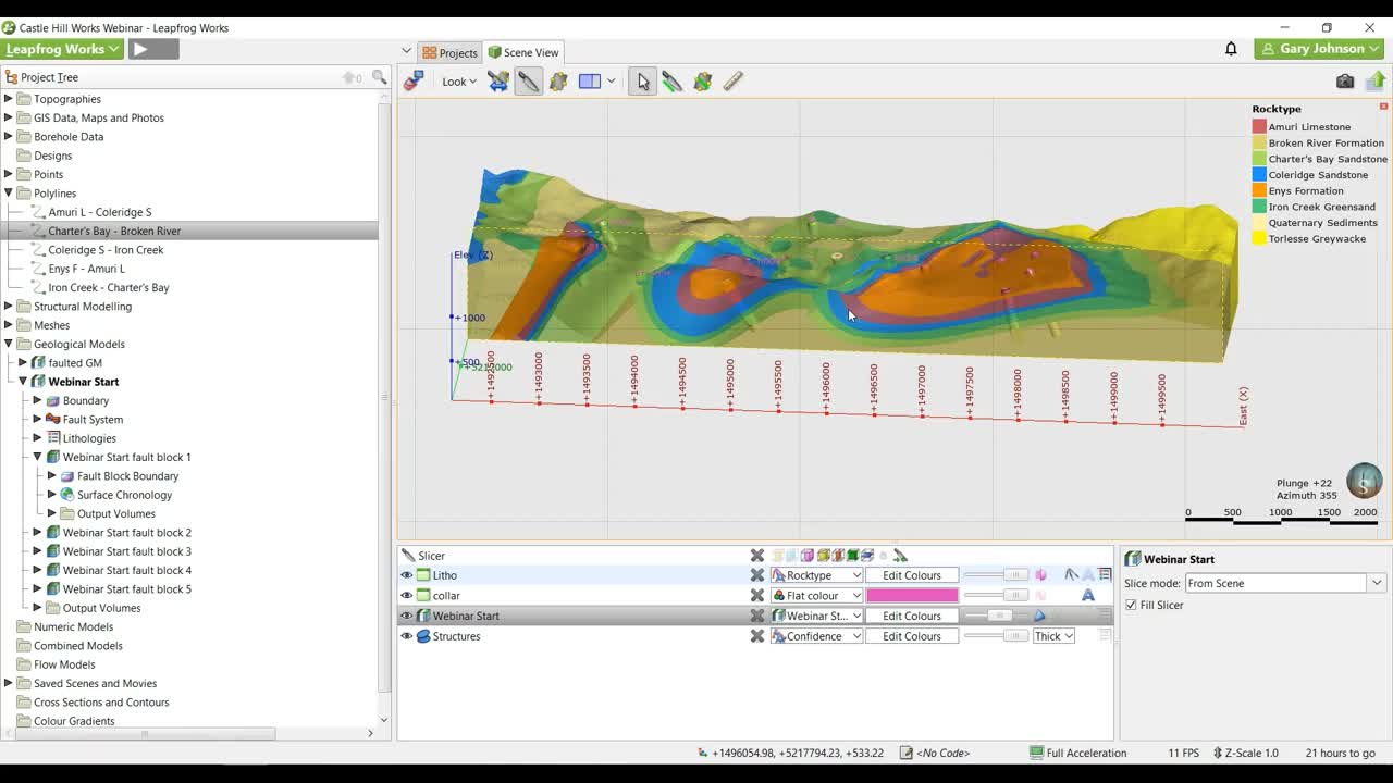
[00:01:20.630]So this is the Leapfrog Works interface.

[00:01:24.731]For those of you who are familiar with Leapfrog Works,

[00:01:26.777]we have our 3D scene here in the middle.

[00:01:28.430]We have our ever important project tree here on the left

[00:01:31.580]and our shape list at the bottom,

[00:01:33.440]which is going to list all of the objects

[00:01:36.100]that are displayed in the 3D scene.

[00:01:38.659]Right here, you can see the finished product

[00:01:41.440]of the model that we will be building today.

[00:01:43.830]And so you can see that this is

[00:01:45.730]a more complex geologic model.

[00:01:53.800]So one of the first things that I want to discuss

[00:01:56.210]are going to be the challenges involved for this model.

[00:01:59.297]And this model incorporates a variety of different data.

[00:02:02.168]First of all, the main data that we’re going to be

[00:02:05.890]focusing on and building the model from is going to be

[00:02:08.140]structural data, which was gathered in a field mapping

[00:02:11.140]survey and some boreholes as well.

[00:02:14.110]In addition, we also have some downhole structural data.

[00:02:18.317]And so if I clear some of these objects out of the scene,

[00:02:21.112]you can see here is our structural data

[00:02:23.200]that was gathered from field mapping.

[00:02:25.060]And then we have some downhole structural data as well.

[00:02:28.070]If you’re wondering what these structural

[00:02:31.380]disks are actually representing,

[00:02:33.000]you can always click on an object in the scene

[00:02:35.910]and a little dialogue box will pop up over here on the left.

[00:02:39.410]So this structural data is just downhole,

[00:02:42.240]dip and as myth and a location in space.

[00:02:45.423]And we also have assigned a polarity,

[00:02:50.530]just to show you what we’re dealing with here.

[00:02:52.980]We also have other data gathered in this project.

[00:02:55.830]And so we actually have of course,

[00:03:00.060]a topography for the site,

[00:03:01.210]but we have a geologic map as well, this is very common.

[00:03:03.760]You might find geologic maps floating out on the internet,

[00:03:07.040]or you might have one from your own field surveys.

[00:03:10.251]In this project we also have applied some manual edits

[00:03:14.300]using polylines to digitize the contacts

[00:03:17.550]of our geologic map.

[00:03:19.230]A lot of times you might build a geologic model

[00:03:21.540]that doesn’t match precisely to your geologic map.

[00:03:25.310]And so this is going to be an option to ensure

[00:03:27.900]that your contacts are precise

[00:03:30.460]and matching your geologic model.

[00:03:35.630]We also then have a few faults, so in this case four faults,

[00:03:40.654]and you know, it was very common.

[00:03:42.690]A lot of the times you might be dealing with, you know,

[00:03:44.790]structural faults and want to incorporate them

[00:03:47.450]into your model to see how they affect the model.

[00:03:49.910]And so that you can work with the individual

[00:03:52.630]fault blocks as well.

[00:03:54.680]And so this is going to be, you know,

[00:03:56.580]some of the challenges that are involved in making this

[00:03:58.600]a more complex model.

[00:04:00.850]And personally, this is one of my favorite models.

[00:04:03.160]I think it brings the whole picture together.

[00:04:06.240]And so you have a bunch of complex data,

[00:04:08.430]as you can see in our all data gathered, saved, seen.

[00:04:13.350]Here, you can see we have a ton of complex data.

[00:04:15.790]How can we bring this to clarity?

[00:04:17.370]How can you demonstrate it?

[00:04:19.290]What is actually in the subsurface?

[00:04:21.420]And so we will be going from this right here,

[00:04:23.840]this collection of data to a 3D geologic model.

[00:04:29.900]So I’m going to go ahead and clear the scene

[00:04:32.300]in the top left here.

[00:04:33.510]It looks like a bucket being thrown on a window

[00:04:36.320]or a desktop.

[00:04:39.270]You might have been wondering how I was just dragging

[00:04:42.250]and dropping those scenes into the 3D scene.

[00:04:45.880]Over here. We do have a saved scenes and movies folder.

[00:04:49.620]This works great if you want to pretty much

[00:04:52.230]collect bookmarks of your model.

[00:04:54.080]And so you can easily drag and drop these scenes

[00:04:58.000]into the 3D scene,

[00:04:59.670]and you will see all of those objects that you’ve saved.

[00:05:02.950]And this can just be done with a right click

[00:05:05.210]on the save scenes and movie and save current scene.

[00:05:08.960]I think that this is great for actually, you know,

[00:05:14.110]being able to walk someone through the different steps

[00:05:16.620]of constructing your model,

[00:05:17.920]or if you have a certain perspective of your model

[00:05:20.290]that you want to save, this is a great way to go about that.

[00:05:27.590]So for this project, we’re going to be building

[00:05:30.120]a new geologic model.

[00:05:31.630]I do want to show you that we have already constructed

[00:05:34.670]this geologic model here in the faulted GM,

[00:05:38.010]but I have now set up a new geologic model called

[00:05:41.277]webinars start, which we have not built any surfaces for.

[00:05:46.900]So I will walk you through the process

[00:05:48.640]of building my different surfaces.

[00:05:53.080]I like to bring my boreholes into the scene

[00:05:56.000]with just my lithology codes on them

[00:05:59.110]while I go through this project.

[00:06:01.516]In this instance, I already have a strap column,

[00:06:05.010]so I already know the age order of my lithologies.

[00:06:08.120]And so I know, you know, what order I’m going to want

[00:06:11.260]to order them in the surface chronology section

[00:06:13.910]of the geologic model over here on the left.

[00:06:18.170]If you have built a geologic model in Leapfrog Works before

[00:06:21.350]then you know that you’re going to be building surfaces

[00:06:24.007]for the geologic model,

[00:06:26.950]which you will then activate to actually build a 3D model.

[00:06:33.410]In past webinars and many instances you might have used

[00:06:36.820]the deposit and erosion functions.

[00:06:39.620]For this example, we will be using structural surfaces.

[00:06:43.900]Structural surfaces are nice because they allow you

[00:06:46.410]to incorporate structural data and borehole contacts

[00:06:50.290]into a single surface.

[00:06:52.790]And just to show you how more geologically realistic

[00:06:56.530]these structural surfaces are compared to a deposit,

[00:06:58.908]here we have both surfaces in the scene

[00:07:02.100]for the same deposit.

[00:07:04.240]I’m going to turn off the structural surface

[00:07:07.613]and you can see here in the scene

[00:07:09.720]that we have a simple deposit.

[00:07:11.930]These deposits are often just going to be planer surfaces.

[00:07:16.280]And so if you have collected structural data,

[00:07:19.280]I always recommend building a structural surface.

[00:07:22.320]This structural surface will allow it to conform

[00:07:25.630]to your different dip and as myth that you have applied

[00:07:28.810]or gathered in your field surveys.

[00:07:32.424]And so this is what we’ll be using in this project

[00:07:34.500]to build the models from.

[00:07:38.450]For speed purposes of building this geologic model,

[00:07:41.552]I have already imported different faults,

[00:07:44.640]which I showed you those four faults earlier.

[00:07:47.860]These I’m going to keep active for the time being.

[00:07:51.025]I’m going to actually build the geologic model first,

[00:07:55.540]construct all of my surfaces,

[00:07:57.490]and then I will apply the faults afterwards

[00:08:00.500]and break it up into fault blocks.

[00:08:03.490]So you can see in parentheses next to each surface,

[00:08:06.190]it’s listed as inactive.

[00:08:08.178]You will actually have to double-click on the fault system

[00:08:11.180]and activate those.

[00:08:14.600]Before I go ahead and build my surfaces,

[00:08:17.160]I’m going to show you a few things that are very important

[00:08:19.650]in the geologic model settings.

[00:08:21.890]So if you right click on your geologic model,

[00:08:23.950]you can always open some edit settings.

[00:08:27.320]And so I’ll bring this into the middle.

[00:08:31.170]For this project, I’m going to keep a resolution

[00:08:33.530]of 50 units, which is going to correspond to the sidelines

[00:08:36.990]and the triangles that are used to build the surfaces.

[00:08:40.580]The most important thing here is the snap to data.

[00:08:43.420]A lot of the time you might be wondering why your contacts

[00:08:46.340]aren’t precisely snapping or why your surfaces

[00:08:49.680]aren’t precisely snapping to your contact points.

[00:08:52.920]That is because you will want to ensure your snap to data

[00:08:55.910]is on by default, it is often off.

[00:08:59.300]If you’re only using boreholes to build your model,

[00:09:03.040]then you’ll want to just use it drilling only.

[00:09:05.390]In this case, we’re going to be using boreholes

[00:09:07.780]and structural data so we want to ensure that that is on

[00:09:10.520]all data as well.

[00:09:12.940]Just something to keep in mind,

[00:09:14.150]if you ever see that your bore holes,

[00:09:15.520]aren’t snapping to your surfaces,

[00:09:18.910]check out your snap to settings.

[00:09:24.460]Okay, and so I’m actually going to go ahead

[00:09:27.100]and start building our surfaces now.

[00:09:31.270]In past experiences,

[00:09:33.300]you might have built your, you know,

[00:09:34.870]your geologic model surfaces from top to bottom,

[00:09:37.274]or from bottom to top, you can do it either way.

[00:09:41.300]In this instance, I’m going to do top to bottom.

[00:09:44.932]And so the first contact that I will be building

[00:09:49.520]is going to be the Ennis formation.

[00:09:53.570]And so down here, we have a new structural surface,

[00:09:56.600]which I will be building.

[00:09:58.350]This will allow you to add structural data here at the top.

[00:10:03.350]So in this case, I’ve already set aside two different.

[00:10:06.330]So we have our field mapping structural data,

[00:10:08.620]and then we have our downhole structural data,

[00:10:12.090]and I’m going to apply both of these to the single surface.

[00:10:17.070]I’m then going to want to actually

[00:10:18.890]select my borehole contacts.

[00:10:20.610]And so if you click on add,

[00:10:21.970]you can add based lithology contacts.

[00:10:24.660]Based ecology contacts is always

[00:10:26.270]going to be referencing your boreholes.

[00:10:30.460]The first lithology or the primary lithology

[00:10:32.930]that I’ll be building here is going to be

[00:10:35.105]the Ennis formation.

[00:10:38.030]The Ennis formation is going to be one of the youngest

[00:10:42.450]surface, so towards the surface.

[00:10:44.060]And so I’m going to be using contacts below.

[00:10:47.311]So just something to keep in mind,

[00:10:49.300]if you’re building from bottom to top,

[00:10:50.980]you’ll probably want to use contacts above.

[00:10:52.760]And if you’re building from top to bottom,

[00:10:54.870]you’ll probably want to use contacts below.

[00:10:58.890]So I’m going to go ahead and press OK.

[00:11:03.510]You will see here that it’s going to list,

[00:11:05.210]the lithology is the first, you know,

[00:11:07.840]younger is the Ennis

[00:11:09.987]and the older is the Amauri limestone, I believe.

[00:11:13.380]And so we’re going to go ahead and press okay for this.

[00:11:20.810]Okay, so we have now built the MRA and Ennis

[00:11:23.740]formation contacts here.

[00:11:25.550]We’re now going to repeat that process

[00:11:27.850]for the next formation, which is the Emory.

[00:11:30.620]So on the left, it’s always going to list the younger

[00:11:33.350]formation or the older formation,

[00:11:35.690]on the right is going to be the younger formation.

[00:11:38.910]So the next formation, that will be our primary lithology.

[00:11:43.040]And so we’re just going, right clicking on the surface,

[00:11:46.641]chronology going back down to new structural surface,

[00:11:49.050]and we’re going to want to add our other sets

[00:11:51.770]of structural data.

[00:11:55.023]I’m going to press okay.

[00:11:55.856]And then we’re going to want to add

[00:11:57.280]the base lithology column.

[00:11:59.490]In this case, we are using the limestone contacts.

[00:12:03.017]One thing that’s nice about a structural surface

[00:12:06.049]is that you can actually apply not just contacts above

[00:12:09.720]or contacts below, but you can also use both.

[00:12:13.047]One thing that you’re going to want to keep in mind

[00:12:17.150]is when you’re building surfaces in Leapfrog Works,

[00:12:19.700]you’re not going to want to repeat

[00:12:21.600]the same borehole contacts.

[00:12:23.910]And so this is a great place to demonstrate

[00:12:27.450]where you’re going to want to ignore a set of contact points

[00:12:30.150]because they’ve already been used.

[00:12:31.950]So because the NS formation and a Maury limestone contacts

[00:12:36.340]have already been formed in the previous surface,

[00:12:38.900]we’re not going to want to reuse the same contact points.

[00:12:42.340]There’s nine locations where the NS formation

[00:12:45.260]is contacting the limestone.

[00:12:47.430]So you can just drag that over

[00:12:49.760]into the ignored lithology section.

[00:12:52.590]You will see me do this a few times

[00:12:54.530]throughout the modeling process here.

[00:12:56.850]And that is because we don’t want to duplicate

[00:12:59.370]any contact points.

[00:13:00.930]We always want to have a single surface

[00:13:03.020]through a single set of contact points.

[00:13:06.730]And so these are going to be our Amaury limestone,

[00:13:10.350]Coleridge sandstone contacts.

[00:13:12.940]I’m going to go ahead and press OK.

[00:13:17.180]And it’s all properly assigned here.

[00:13:19.730]I’m going to go ahead and press okay again.

[00:13:26.950]So some of you might be wondering how the structural data

[00:13:30.807]takes into account which lithology is there.

[00:13:33.850]And so this is a great time to point this out.

[00:13:36.676]And so if I open up my structural modeling folder,

[00:13:39.930]you can see that we have this field mapping structures.

[00:13:43.110]I’m going to drag that into the scene.

[00:13:46.040]You can see in the top, right,

[00:13:47.650]your go-to webinar panel might be hiding it.

[00:13:49.810]So it’s over here.

[00:13:51.220]But you can actually apply lithologies or categories

[00:13:55.750]to structural data for modeling purposes.

[00:13:58.680]And so here you can see that our structural data

[00:14:01.340]is actually assigned by rock type.

[00:14:04.270]So you can, you know,

[00:14:05.820]if you want to assign a rock types to structural data,

[00:14:09.110]you can easily do that within a CSV.

[00:14:12.087]And, you know, just when you’re importing

[00:14:14.710]that structural data, assign that column as a lithology

[00:14:18.200]or as a category.

[00:14:22.090]So I’m going to clear the scene

[00:14:23.230]and I’m going to keep building my surfaces.

[00:14:25.570]One thing to keep in mind is when you’re building

[00:14:27.740]from top to bottom, the surfaces aren’t going to come in

[00:14:31.790]in the correct order.

[00:14:32.860]And so you can double-click on your surface chronology

[00:14:35.969]to open up the actual chronology section,

[00:14:40.350]which is pretty much a strap column,

[00:14:42.830]and you can move that surface down one.

[00:14:45.960]We know that the collared sandstone Marie limestone contact

[00:14:48.790]is older than the previous.

[00:14:50.656]So we want to move them down as we go through the model.

[00:14:55.170]And so you can see over here on the left that it has now

[00:14:57.970]reordered those contacts.

[00:15:01.890]I’m going to go through and then build

[00:15:03.640]the next set of contact points.

[00:15:07.020]So from my Strat column and knowledge of the site,

[00:15:09.860]I know that the next formation in my strategraphy

[00:15:14.180]is going to be the iron Creek,

[00:15:17.585]the iron Creek contacting the Coleridge sandstone.

[00:15:22.240]So the colored sand stone on top iron Creek on the bottom,

[00:15:25.930]I’m going to go ahead and add that structural data again

[00:15:28.410]to the surface.

[00:15:30.200]And I’m now going to add my base lithology contacts.

[00:15:34.870]So the primary lithology here,

[00:15:37.860]the next in our sequence is the cord sandstone.

[00:15:40.780]We’re going to want to use contacts below

[00:15:42.620]as we’re building from top to bottom.

[00:15:45.020]So this contact point is going to be

[00:15:47.390]our Coleridge sandstone and iron Creek green sand.

[00:15:50.970]This one contact point of more limestone is going to be

[00:15:53.990]another duplicate point that can be an ignored lithology.

[00:15:57.490]We want to set up the contacts just between the colored

[00:16:00.470]sand stone and the iron Creek green sand.

[00:16:03.980]And so once again, we’re going to accept

[00:16:06.640]the default settings and go ahead and press, okay.

[00:16:11.550]You can see the Coleridge is younger

[00:16:13.050]and the iron Creek is older.

[00:16:14.770]Everything looks good here,

[00:16:16.410]can go ahead and press okay again.

[00:16:30.140]So we now made that next surface.

[00:16:32.510]I’m going to once again, reorder that

[00:16:35.160]so that I’m keeping track.

[00:16:36.440]And I like to do this as I’m coming through the model,

[00:16:38.780]because it allows you to actually keep track of, you know,

[00:16:42.450]as you’re building the surfaces, what’s older,

[00:16:43.960]what’s younger so this is the oldest contacts.

[00:16:45.970]So I’m going to want to move it down to two spots

[00:16:48.470]and just press, okay.

[00:16:51.800]The next formation that we want to build

[00:16:53.890]is going to be the primary pathology of the iron Creek,

[00:16:56.880]which is contacting the charters at bay formation.

[00:17:03.500]So we’re just repeating this process

[00:17:05.160]of adding the structural data to each surface,

[00:17:09.510]and then we’re going through

[00:17:10.390]and adding the borehole contacts.

[00:17:13.400]The primary lithology here is going to be

[00:17:16.069]the iron Creek green sand.

[00:17:19.470]We want to use the contacts below

[00:17:21.559]and we want to ignore these single contact points,

[00:17:24.910]which are also going to be duplicates.

[00:17:28.030]So we’re just creating a surface for the iron Creek

[00:17:30.470]green sand and the charters bay sandstone.

[00:17:38.720]Going to go ahead and press okay again.

[00:17:44.920]Okay, so we’ve now built the next surface.

[00:17:47.250]I’m going to move that down again as well,

[00:17:50.150]just making it the oldest surface and going to press, okay.

[00:17:55.130]We now have our last contact to set up.

[00:18:00.040]And so that is going to be our charters bay

[00:18:03.090]and broken river contacts.

[00:18:05.830]I’m going to go ahead and add the structural data again.

[00:18:09.227]And I’m going to add the base lithology contacts.

[00:18:14.810]So the charters bay is the primary reason contacts below,

[00:18:21.550]and we want to just set up the broken river formation

[00:18:24.465]and the charters bay,

[00:18:26.050]which those contact points have not been used yet.

[00:18:30.110]I’m going to go ahead and press okay.

[00:18:32.290]And okay.

[00:18:40.830]So now I want you to just ensure that my surface chronology

[00:18:44.150]is in the correct order in some of the move

[00:18:46.350]everything down, that looks good.

[00:18:51.770]Now it comes a time where you might be looking

[00:18:54.080]at your surface chronology, or you might have,

[00:18:57.260]for example, a geologic map,

[00:18:59.640]and you compare your contacts to your geologic map,

[00:19:04.290]and you might see that those do not match precisely.

[00:19:07.500]Right now we have not activated the surfaces yet.

[00:19:09.990]So if we drag over this little thing,

[00:19:12.150]you could see those are still listed as inactive.

[00:19:14.945]That is because before activating these surfaces,

[00:19:18.780]I’m going to want to make some polyline edits.

[00:19:21.720]This is often the time consuming part of the project,

[00:19:25.210]where you have to go in and make some manual manipulations

[00:19:28.491]to allow your surfaces to conform to your geologic map.

[00:19:33.170]For this project, we have already created polylines

[00:19:35.852]that will allow our surfaces in this case to match

[00:19:42.580]our geologic map.

[00:19:44.150]So if we place our geologic map in there,

[00:19:45.814]one little tips and tricks,

[00:19:48.783]if you double-click on any object,

[00:19:50.040]it will highlight all like objects.

[00:19:51.690]So in this case, all of our surfaces,

[00:19:53.260]and you could turn them all off at once.

[00:19:56.286]And then you can also press a D on the keyboard

[00:19:59.010]to look directly down.

[00:20:02.130]We’ve made some polylines in this project that outline

[00:20:04.900]some of the contacts.

[00:20:07.190]So in addition to, you know, structural data and boreholes,

[00:20:10.440]we’re also adding manual manipulations or polylines

[00:20:13.377]in this case to the contacts themselves.

[00:20:17.400]And so this will often be done after you’ve built

[00:20:19.940]all of your contacts, and you realize that, you know,

[00:20:22.440]maybe there’s some locations where it’s not matching

[00:20:25.080]as you would like.

[00:20:26.220]And so that’s why I’m going to do or add these polylines

[00:20:29.250]after the fact that I’ve already created all of my surfaces.

[00:20:34.190]And though this is just something to keep in mind

[00:20:35.740]that you can do this.

[00:20:37.230]Personally, I like to use, and you can see here 3D points.

[00:20:42.020]And so those are generated in the polylines folder.

[00:20:45.620]The points are nice because they don’t have 3D tangents

[00:20:50.310]that polylines have, and it makes it easier

[00:20:52.990]to model contacts, for example, or digitize a geologic map.

[00:20:59.340]And so I’m just going to go ahead and clear my scene.

[00:21:03.100]I’ve named all of my polylines

[00:21:05.270]according to the actual contacts.

[00:21:08.370]And so that makes it easy to apply them to each surface.

[00:21:12.180]And so if I’m looking for my, you know,

[00:21:14.357]Murray limestone and its formation contacts,

[00:21:16.860]so you can see that I have a poly not line named,

[00:21:19.410]and it’s an Amaury.

[00:21:21.080]And so if you want to add any data to any surface

[00:21:24.730]in Leapfrog Works,

[00:21:25.680]you can right click on that surface and go up to add,

[00:21:29.850]you can see a variety of different objects that you can add

[00:21:32.270]to surfaces, GIS data included, points,

[00:21:35.360]other borehole contacts,

[00:21:36.760]in this case, polylines is what we’re looking for.

[00:21:41.070]So we’re doing the Amaury and Ennis.

[00:21:42.900]So we want to select the NSA memoria

[00:21:45.750]and add those polylines.

[00:21:55.240]So if I expand the surface, you can now see that those

[00:21:58.746]polylines have been added to that surface.

[00:22:03.650]I’m going to go ahead and repeat that

[00:22:07.690]for the rest of my surfaces,

[00:22:09.074]as I have a polyline contact for each.

[00:22:11.690]So we’re doing the Coleridge Maury.

[00:22:14.230]So I want to find that Maury Coleridge polyline.

[00:22:17.950]And I want to add that to that surface.

[00:22:25.240]Just to show you that you can do multiple processes at once,

[00:22:29.490]so while this remains processing,

[00:22:32.155]you can go ahead and add multiple other surfaces

[00:22:34.980]or multiple other additions, or polylines in this case

[00:22:37.580]to your surfaces while it’s processing.

[00:22:40.140]So I’m going to go ahead and complete the rest

[00:22:42.320]in one single step.

[00:22:44.920]So I’m going to add the polylines

[00:22:46.230]for the iron Creek Coleridge.

[00:22:48.140]So Coleridge iron Creek.

[00:22:50.869]I’m going to go ahead and press, okay.

[00:22:53.493]Then repeat the process for the charters bay.

[00:23:19.707]So in broken river Charter’s bay.

[00:23:23.268]I’m going to add the final polyline,

[00:23:26.712]charges bay broken river.

[00:23:27.553]You’re going to go ahead and press, okay.

[00:23:33.260]So we’ve now added all of our polylines

[00:23:36.280]to all of our surfaces.

[00:23:38.070]We’ll now want to actually go through

[00:23:40.340]and activate all of those surfaces.

[00:23:43.110]So you might look at your model now

[00:23:45.560]and wonder why is it still unknown?

[00:23:48.920]That is because Leapfrog keeps surfaces inactive

[00:23:52.140]until you activate them.

[00:23:54.150]In order to activate them,

[00:23:56.110]you’re going to want to double-click on the surface

[00:23:58.820]chronology folder or curved surface chronology section,

[00:24:02.206]and tick the little box next to contacts surface,

[00:24:07.361]and you can go ahead and press, okay.

[00:24:10.784]And that will process the model

[00:24:12.640]and build the output volumes for you.

[00:24:18.240]So the model has now processed.

[00:24:21.370]You can now see that we have output volumes generated,

[00:24:24.288]and if we want it to slice through this model,

[00:24:27.713]let’s press D on the keyboard and get the slicing tool out.

[00:24:32.288]You can see that we have some nice folds in there,

[00:24:36.600]but the one thing that we haven’t incorporated

[00:24:38.820]into this model yet is going to be the fault systems.

[00:24:42.450]In this case, we have four different faults

[00:24:44.280]which were imported into the meshes folder

[00:24:47.090]and then use to build faults.

[00:24:50.455]I have already imported these faults

[00:24:53.380]into this fault system section here.

[00:24:55.890]If you want to add any faults to a model,

[00:24:58.330]you would just right click on the fault system

[00:25:00.840]and go to new fault.

[00:25:02.400]And you can see that there’s a variety of options here

[00:25:04.720]that you can build faults from.

[00:25:07.497]Activating faults is very similar

[00:25:10.390]to the process of activating your surfaces.

[00:25:14.540]And so I’m going to double-click on the fault systems

[00:25:17.180]section of the geologic model,

[00:25:19.400]and I’m going to tick the little box next to the faults.

[00:25:24.000]One thing to keep in mind at this stage is that your faults

[00:25:27.060]are similar to your surfaces and that they have to be

[00:25:29.820]in the correct age order that they occurred.

[00:25:32.570]For example, if you have faults cutting through each other,

[00:25:35.004]you can then assign interactions down here

[00:25:38.720]of your fault system.

[00:25:39.920]And so you can allow terminations,

[00:25:41.720]all of that good stuff as well.

[00:25:44.903]I’m going to go ahead and activate my faults

[00:25:46.090]and by pressing okay.

[00:25:59.600]So the model has now processed.

[00:26:01.340]It has incorporated some of these faults into the system.

[00:26:04.330]One thing that I’m going to want to check now

[00:26:06.432]is double check that we have the correct order

[00:26:09.860]of our faults, so the Cheeseman fault, the flock hill,

[00:26:13.310]Craig Bern and Sugarloaf all correctly ordered.

[00:26:17.059]One thing that jumps right off to me is that I have

[00:26:20.270]this section that is assigned as unknown.

[00:26:23.900]That is occurring because in that section

[00:26:26.720]of the fault block,

[00:26:27.920]we don’t have any borehole lithologies identified.

[00:26:32.181]And so there’s actually a borehole in this project

[00:26:35.616]that is listed as just unknown.

[00:26:40.620]And so if I bring these boreholes in, you can see over here,

[00:26:44.885]this borehole is listed as a lithology

[00:26:48.570]that was not have had a surface built for it.

[00:26:50.900]So we didn’t build a surface for the single lithology.

[00:26:53.330]And it’s also only contained in a single fault block.

[00:26:57.490]If I bring that fault block into the scene,

[00:26:59.658]you could see that it’s designated as unknown.

[00:27:04.250]One really easy way to build a surface for this

[00:27:07.740]or build a deposit for this would be well, actually,

[00:27:12.390]it’s probably good to show you how to that the surface,

[00:27:14.730]the model itself is broken up into individual fault blocks.

[00:27:18.330]And so here we have this webinar start model.

[00:27:22.700]I’m actually going to do a little tips and tricks

[00:27:24.420]by right clicking on the project tree

[00:27:25.940]and collapsing it and just expand it.

[00:27:27.952]Only my geologic models folder and our webinar model.

[00:27:32.600]You can see, we have different fault blocks.

[00:27:34.900]In this case, the empty fault block is fault block one.

[00:27:39.210]Each fault block will have its own boundary settings

[00:27:41.530]and its own surface chronology.

[00:27:43.280]So you can actually add surfaces

[00:27:44.860]to an individual fault block,

[00:27:46.730]and then you can actually copy the chronology

[00:27:48.750]of that fault block to another fault block.

[00:27:51.440]So instead of doing what I did and activating the faults

[00:27:54.530]afterwards, you can actually build it by fault block,

[00:27:57.850]by fault block, and then copy chronology

[00:27:59.680]to the rest of those.

[00:28:02.760]In this case, we want you to just assign a lithology

[00:28:04.870]to that fault block.

[00:28:06.660]really easy way to do that is right here

[00:28:08.420]on the background lithology you can assign this.

[00:28:11.310]We know that it’s the twirlies gray whack.

[00:28:14.370]I think that’s how you pronounce that.

[00:28:16.394]That is going to be our background lithology.

[00:28:20.240]And so we’re going to go ahead and just assign that

[00:28:22.640]and go ahead and press OK.

[00:28:39.460]So we now have assigned that lithology

[00:28:41.740]and we have actually completed our geologic model.

[00:28:48.950]You can see that it does confine to the different polylines.

[00:28:52.000]And so if I wanted to bring in some of these contacts,

[00:28:54.669]you can see that those contacts do conform.

[00:29:00.730]And so I think that that’s a cool thing to demonstrate,

[00:29:03.160]the ability to digitize contact lines.

[00:29:06.290]For now, I’m going to clear those from the scene.

[00:29:11.260]And this is the point where you might want

[00:29:13.350]to just confirm your results, you know,

[00:29:16.720]does our model match results easy way to do that would be

[00:29:19.990]to press D on the keyboard and use the slicing tool,

[00:29:23.880]the tool bar at the top and slice, you know,

[00:29:26.580]let’s say lengthwise across the model.

[00:29:29.783]Now you can see, you can’t see through the model.

[00:29:32.280]So if you want it down here in the shapes list

[00:29:34.160]at the bottom, you can highlight your geology interval table

[00:29:38.874]and turn the opacity of that down.

[00:29:42.220]Actually, in this case, we’ll probably want to turn

[00:29:44.842]our geologic model opacity down.

[00:29:48.300]So that webinars start model.

[00:29:50.240]We could turn that down a little bit

[00:29:52.760]and we can zoom in on these different porthole contacts.

[00:29:55.280]And you can see that these boreholes are conforming

[00:29:58.810]or the surfaces are conforming to the boreholes.

[00:30:02.520]And so if we step through the model using the greater than

[00:30:05.910]or less than symbol on your keyboard

[00:30:08.020]or the period in the comma, you can step through the model.

[00:30:12.040]You can see the faults and folds

[00:30:14.130]that it does conform to our boreholes,

[00:30:16.741]and you can see the actual structure of the geology.

[00:30:21.087]A nice thing is there’s many different settings

[00:30:23.840]for the actual slicing tool.

[00:30:26.480]So if you want it to remove the back of the model,

[00:30:29.110]you can do that.

[00:30:30.920]Change the opacity a little bit

[00:30:32.390]to make it a little more visible.

[00:30:35.472]One thing that I’ve seen already arise in the questions

[00:30:39.810]panel down here is why didn’t you model

[00:30:43.449]the quaternary sediments?

[00:30:45.861]And that is a great question.

[00:30:47.960]And so if I’m just looking at my boreholes,

[00:30:50.530]you can see in some of my boreholes,

[00:30:52.688]there is this object that coronary sediments at the top,

[00:30:56.780]in this case, the interval was so tiny and so small

[00:31:00.830]that we didn’t even model it.

[00:31:02.167]And it was only included in a few boreholes

[00:31:05.228]and in some instances only a meter thick.

[00:31:07.500]And so it wasn’t important or relevant

[00:31:09.690]to this geologic model.

[00:31:11.420]A lot of times you might be dealing with deep subsurface

[00:31:14.130]issues and you might want to ignore, you know, upper layers.

[00:31:17.980]That is something that can be done.

[00:31:21.590]<v Mikayla>Thank you, Gary.</v>

[00:31:22.910]All right, we’re now going to begin answering the questions

[00:31:25.160]submitted during today’s presentation.

[00:31:28.230]All right, our first question comes from Kyle.

[00:31:32.580]Kyle asks, why aren’t my surfaces snapping

[00:31:35.930]to the borehole contacts?

[00:31:38.940]<v Gary>This is a great question</v>

[00:31:40.150]and something that arises normally when you’re first

[00:31:42.710]building your surfaces, or, you know,

[00:31:44.740]at any point in your geologic modeling stage,

[00:31:47.540]in the geologic model, you can right click and open,

[00:31:50.798]and you will see that there’s that snap to data setting,

[00:31:54.640]which I referenced earlier.

[00:31:55.770]You want to ensure that that’s on all data

[00:31:57.680]if you’re using more than four holes

[00:31:58.940]or drilling only if you’re only using drilling data.

[00:32:02.230]Another thing to keep in mind is you might often have

[00:32:04.810]vertical exaggeration on which you can turn on down here

[00:32:07.170]in the bottom right.

[00:32:08.620]A vertical exaggeration will make it sometimes appear

[00:32:11.290]that your contacts aren’t going through the right spots.

[00:32:14.320]So sometimes turning that down to one can help.

[00:32:17.650]Another thing to keep in mind is that your boreholes

[00:32:20.345]are often quite wide.

[00:32:22.490]So in this case, they’re probably,

[00:32:24.070]for visualization purposes, I’ve made them quite wide,

[00:32:27.172]you know, 10 meters sometimes.

[00:32:29.550]And of course your core sample that you’ve retrieved

[00:32:32.770]might only be, you know, 10 centimeters thick in diameter.

[00:32:37.670]And so the actual contact point might visually appear

[00:32:40.880]to not be in the correct spot, but it normally is.

[00:32:43.382]And it’s easy to see if you turn the different triangles on,

[00:32:48.240]on the surface, you can see that there’s going to be

[00:32:50.180]a vertex in that contact point.

[00:32:54.730]<v Mikayla>Okay.</v>

[00:32:56.850]All right, the next question comes in from Zoe.

[00:33:02.560]She asks, what if I don’t want my model to be confined

[00:33:05.644]to a rectangle or square?

[00:33:09.270]<v Gary>This is another question that comes up quite often.</v>

[00:33:11.430]A lot of times you might see a Leapfrog model

[00:33:13.610]and it is a square or rectangle.

[00:33:15.880]You can always right click on the boundary section

[00:33:18.890]of the geologic model and add a new lateral extent,

[00:33:22.320]which is going to confine the model by one of these options.

[00:33:26.999]One thing to keep in mind is that you will want

[00:33:28.000]that boundary or lateral extent to be contained

[00:33:31.320]within your topography.

[00:33:36.890]<v Mikayla>Okay.</v>

[00:33:39.710]All right, here’s another question coming in from Nicholas.

[00:33:44.296]He asks, I have a very complicated fault system.

[00:33:48.700]How do you handle faults terminating it against each other?

[00:33:53.799]<v Gary>That is a great question.</v>

[00:33:54.890]So in the fault system, section of the geologic model,

[00:33:57.803]you can assign terminations.

[00:34:00.140]If you have faults that touch each other

[00:34:02.290]or interact with each other,

[00:34:03.550]so you can allow them to cut through each other

[00:34:05.300]or terminate against each other.

[00:34:07.388]If you have a fault that you don’t want to cut through

[00:34:10.070]the entirety of the model, what I’ll often do is build a,

[00:34:13.840]what I like to call a dummy fault,

[00:34:15.510]which I allow the fault to terminate against,

[00:34:17.820]but I keep it inactive.

[00:34:20.510]And so that’s one thing to keep in mind

[00:34:22.040]is you can keep faults inactive,

[00:34:23.680]but allow them to terminate against each other.

[00:34:29.480]<v Mikayla>All right, let’s see.</v>

[00:34:33.148]All right, got another question from Michael who asks,

[00:34:37.393]how would one analyze the structural data

[00:34:40.690]within Leapfrog Works?

[00:34:42.600]<v Gary>So that’s a really good question.</v>

[00:34:44.090]So we do have a ton of structural data in this project

[00:34:46.940]that was gathered in a field mapping survey.

[00:34:50.360]This structural data, if you click on one of the objects,

[00:34:52.440]you can see it’s just a location dip as myth polarity.

[00:34:55.760]And we’ve also assigned lithologies to that.

[00:34:59.020]Within Leapfrog Works, you can create stereo nets.

[00:35:01.690]And so I think staring that’s a really good way

[00:35:03.830]to analyze your data.

[00:35:05.809]In this case, we’ll probably want to open up

[00:35:08.270]the stereo net settings.

[00:35:10.720]And you can see here that you can generate a variety

[00:35:13.070]of different stereo nets in Works.

[00:35:15.640]If I click on the options here,

[00:35:17.030]you can see different stereo net types, projection types,

[00:35:21.800]and there’s a ton that you can do here

[00:35:25.240]for visualization purposes.

[00:35:28.010]Definitely worth experimenting with

[00:35:29.510]if this is something that you deal with.

[00:35:32.600]Structural data is very common in this industry.

[00:35:39.406]<v Mikayla>A question in from Justin who asks,</v>

[00:35:44.060]I often have to export into Modflow V-flow

[00:35:47.409]and other flow modeling packages.

[00:35:50.220]How could I incorporate faults into a flow model

[00:35:55.020]generated in Leapfrog?

[00:35:57.960]<v Gary>It’s another great question.</v>

[00:35:58.793]So flow models we’ll often want to incorporate

[00:36:01.760]some kind of faulting.

[00:36:03.460]Often, you know, these are going to be your flow zones.

[00:36:05.649]The best way to do it currently is going to be using

[00:36:09.270]a vein as the surface for the fault,

[00:36:12.880]and maybe restricting, you know,

[00:36:14.130]the vein allows you to restrict the minimum

[00:36:16.820]or maximum thickness.

[00:36:18.630]So that’s how I would recommend building a vein

[00:36:20.720]for your fault as the best method to do that.

[00:36:28.090]<v Mikayla>Excellent.</v>

[00:36:29.940]Another question coming in from Emma,

[00:36:32.240]what do your structural data tables look like

[00:36:35.730]as in your raw data?

[00:36:37.970]<v Gary>Oh, awesome.</v>

[00:36:39.412]So, you know, if you guys are now interested

[00:36:41.460]or if you have imported structural data or unsure of how,

[00:36:45.250]what you need included,

[00:36:47.000]you can always double-click on any object

[00:36:49.510]that you’ve imported as like a CSV, for example,

[00:36:52.167]and it will actually bring open the table that was imported.

[00:36:56.440]So in this case, the structural data

[00:36:58.270]was just as a simple CSV, so within Excel.

[00:37:01.500]And it’s just an X, Y, and Z location,

[00:37:04.720]a dipping angle and a dipping direction, or the asthma,

[00:37:08.750]the polarity, so which is up or down kind of thing.

[00:37:13.040]And then we also then here assigned a rock type,

[00:37:16.295]an area and faulting.

[00:37:19.490]Rock type, area, and faulting can all be imported

[00:37:23.220]as a category rock type.

[00:37:24.590]Of course you can also import as a lithology.

[00:37:32.657]<v Mikayla>All right, our next question,</v>

[00:37:35.460]coming in from Jenny who asks,

[00:37:38.330]we often deal with a lot of data for our sites

[00:37:41.670]with 2000 boreholes or more spanning many miles,

[00:37:45.680]how large is this site for the model you built?

[00:37:49.410]<v Gary>So, yeah, so a lot of the times you might have</v>

[00:37:51.570]a site that is multiple kilometers long.

[00:37:55.300]And one thing to also keep in mind is that Leapfrog Works

[00:37:58.500]is unitless, so when I actually show you these units,

[00:38:01.585]I know that they are in meters.

[00:38:03.870]So just these are going to be meters.

[00:38:06.000]We do have a ruler tool at the top that you can use

[00:38:09.970]to measure any objects in your 3D scene.

[00:38:12.380]So I’m going to go, just go across lengthwise and width wise

[00:38:15.040]and see how big this site is.

[00:38:18.270]It’s about eight kilometers long,

[00:38:20.750]and it is about three and a half kilometers wide.

[00:38:25.620]So about eight kilometers by three and a half kilometers,

[00:38:28.760]which I would consider, you know,

[00:38:31.840]about an average size site.

[00:38:34.140]A lot of times I see products that are only maybe

[00:38:36.360]a few hundred meters across,

[00:38:38.050]but also I’ve seen projects that are 80 kilometers

[00:38:41.250]by 40 kilometers, so the fact that it is unitless

[00:38:44.750]actually allows it to build

[00:38:46.310]much larger project sizes or extents.

[00:38:53.590]<v Mikayla>Okay.</v>

[00:38:54.710]All right, we have time for one more question.

[00:38:59.100]This final question comes in from Jeremy.

[00:39:02.760]How would you share your results of the model with others?

[00:39:07.750]<v Gary>So, yeah, that’s a great question.</v>

[00:39:09.880]There’s a variety of different tools in Works

[00:39:11.910]that allow you to share your results.

[00:39:15.930]Of course, we have cross-section tools where you can

[00:39:19.710]generate a variety of different cross-section types,

[00:39:22.170]which can be included in presentations.

[00:39:24.430]We also have saved scenes in movies

[00:39:27.130]where you can save scenes and generate a movie from them.

[00:39:30.292]I am not a videographer, but I can actually build

[00:39:35.360]a pretty good movie within Leapfrog.

[00:39:36.950]It makes it very straightforward.

[00:39:39.788]And of course we have free viewing platforms

[00:39:43.510]which are Leapfrog View and Leapfrog Viewer,

[00:39:46.430]where you can easily upload your scenes and your 3D objects

[00:39:51.686]to a cloud-based platform where you can share them

[00:39:57.170]with your colleagues or clients.

[00:39:59.100]And these are free platforms

[00:40:00.740]and you can share them with anyone.

[00:40:02.780]So here you would just choose, you know,

[00:40:04.260]the upload option in my web browser.

[00:40:08.560]I then have my dashboard where I have my 3D scene,

[00:40:12.400]where you can create slides or slideshows

[00:40:16.530]and walk someone through the story of your project.

[00:40:19.220]And you can then easily share this with collaborators

[00:40:22.723]and you can control their, you know,

[00:40:25.910]how much are they just a viewer,

[00:40:27.580]can they edit and make slides?

[00:40:30.760]You can share this with the link

[00:40:32.560]and you can also now embed this publicly in a webpage.

[00:40:35.700]So if you want it to publicly embed a model and/or provide,

[00:40:40.300]you know, put this on LinkedIn or, you know,

[00:40:42.010]put a 3D model on LinkedIn, you can easily do that now,

[00:40:44.620]which is pretty cool.

[00:40:47.940]I’m going to cancel that.

[00:40:50.170]<v Mikayla>So thank you, Gary.</v>

[00:40:51.520]And thank you everyone for attending today’s webinar,

[00:40:54.800]Leapfrog Works Best Practice for Modeling Complex Geology.

[00:40:59.120]If you have any other questions,

[00:41:00.700]please contact our technical support team

[00:41:03.050]at [email protected].