Leapfrog Works Best Practice – Building A 3D Model From A Geologic Map

In this webinar we will cover:

• Visualising and analysing data in Leapfrog
• Build a geologic model from topographical map and structural discs (no boreholes required)
• Share results using Seequent View

Overview

Video Transcript

[00:00:00.781]<v McKayla>Good morning, everyone.</v>

[00:00:01.690]And welcome to today’s webinar,

[00:00:03.410]Best Practice for Building a Geological Model From a Map.

[00:00:08.310]I would now like to introduce Gary Johnson,

[00:00:11.130]sequence customer solutions specialist,

[00:00:13.420]and your main technical support resource.

[00:00:15.990]Gary is located in our office in Broomfield, Colorado,

[00:00:19.130]and has a geology background.

[00:00:24.120]<v Gary>Thank you, McKayla.</v>

[00:00:25.770]Today, I’m looking forward to taking you through the process

[00:00:28.370]of building a geologic model from a geologic map.

[00:00:32.570]For today’s agenda, we will first be visualizing

[00:00:35.450]and analyzing the data in Leapfrog.

[00:00:38.380]This includes structural data, GIS data,

[00:00:41.480]a topography that has been imported, and a geologic map,

[00:00:45.550]which we’ll be using to construct our model.

[00:00:48.210]We will then actually walk through the process

[00:00:50.280]of building the geologic model in Leapfrog.

[00:00:53.280]We’ll discuss different ways to share your results,

[00:00:56.360]and we’ll leave some time for questions at the end.

[00:01:00.140]I will now jump into Leapfrog Works,

[00:01:02.917]and begin the modeling process.

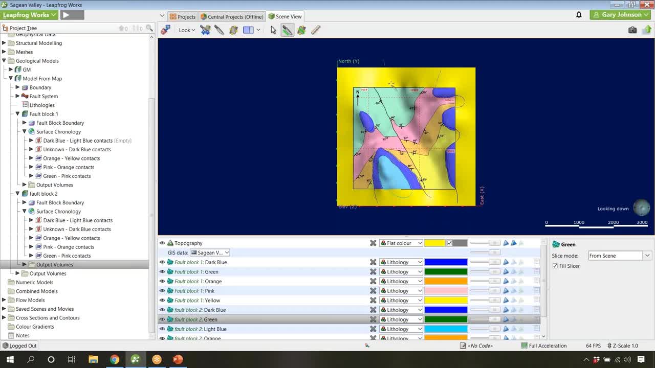
[00:01:08.970]For those of you who are familiar with Leapfrog Works,

[00:01:11.330]this is the user interface.

[00:01:14.040]This includes the ever important project tree on the left,

[00:01:18.180]the scene view in the middle,

[00:01:19.410]where you can interact and view objects in 3D,

[00:01:22.820]the shape list at the bottom,

[00:01:24.720]the shape list is going to list any objects

[00:01:26.840]that are then included in the 3D scene.

[00:01:29.460]For example, if I bring in a topography,

[00:01:32.300]you can see it then pops up in the shape list at the bottom.

[00:01:36.210]The shape list is nice because this is where

[00:01:37.920]you’re going to be controlling your visualization settings,

[00:01:40.560]whether you want to display a map on your topography,

[00:01:42.940]change the opacity, all of the visualization settings

[00:01:46.790]that are here included at the shape list.

[00:01:48.840]We then have some additional options

[00:01:50.530]if you click on an object in the shape list,

[00:01:52.930]in the properties panel in the bottom right.

[00:01:58.120]Now, I know I mentioned the project tree is very important.

[00:02:01.210]The project tree was also designed to match your workflow

[00:02:03.850]in a top-down approach.

[00:02:05.920]The project tree begins with topographies folder,

[00:02:09.220]GIS data maps and photos.

[00:02:11.740]These are going to be your more common inputs.

[00:02:15.060]In the center, we have our actual modeling folders,

[00:02:18.220]and at the bottom of the project tree,

[00:02:19.690]we have some common outputs such as save scenes and movies,

[00:02:22.750]cross sections and contours.

[00:02:25.010]And we’ll walk you through the process

[00:02:26.500]of going through the product tree

[00:02:28.040]and constructing your model, and then putting some outputs.

[00:02:36.910]The first data that was imported into this project

[00:02:39.260]to actually construct the model, was the typography.

[00:02:42.750]The typography was brought in as points via a CSV file,

[00:02:46.880]but this could also be a DEM or a variety

[00:02:49.330]of different surface types, whether it’s an elevation grid,

[00:02:52.630]or a common mesh format from an AutoCAD program.

[00:02:58.090]We also imported some GIS lines in this project.

[00:03:01.670]The GIS data was used to actually build the model,

[00:03:05.550]which is not always so common,

[00:03:07.710]but I like to show that this is a possibility here.

[00:03:12.670]Of course, we were using a geologic map

[00:03:15.070]to actually build the basis of this model.

[00:03:17.497]And so, here you can see the geologic map that was used.

[00:03:21.110]This includes some structural contact data.

[00:03:24.800]One thing to note that this contact data,

[00:03:27.360]or that the structural data is on contact.

[00:03:30.810]And so, these contact locations and structural information

[00:03:35.030]including dip and dipping angle, were used

[00:03:37.950]to actually build the surfaces of this geologic model.

[00:03:40.960]And I will take you through that process shortly.

[00:03:46.740]Now, one little tips and tricks.

[00:03:49.300]If you ever have objects in the scene,

[00:03:51.580]and you wish to eliminate those from the scene

[00:03:53.550]and restore them back to the project tree,

[00:03:55.890]we have this nice little clear scene tool right here.

[00:03:58.930]The clear scene tool

[00:04:00.230]doesn’t delete anything from the project.

[00:04:02.200]It just restores it back to the project tree.

[00:04:04.810]Now, if you ever wanted to save what you’re looking at

[00:04:07.360]in the 3D scene, that’s where

[00:04:09.350]the save scenes and movies folder comes in handy.

[00:04:12.300]You can always right click, and save your current scene.

[00:04:17.400]This allows you to always restore back to that perspective,

[00:04:20.530]as you’ve seen,

[00:04:21.363]I just dragged and dropped this into the scene,

[00:04:24.320]and will always return you to that perspective.

[00:04:27.650]So no worries about having to navigate back

[00:04:29.950]to a certain perspective, and/or having

[00:04:32.630]to bring all of those objects back into the scene,

[00:04:35.440]utilize the save scenes folder, and this will do it for you.

[00:04:38.210]And it almost acts as a bookmark.

[00:04:43.610]One thing that I think is worth mentioning

[00:04:45.220]at this point in the project

[00:04:46.410]is that there are no boreholes included in this model.

[00:04:50.470]The most common format

[00:04:51.640]to actually construct models in Leapfrog Works

[00:04:54.619]is probably boreholes in my experience.

[00:04:57.860]But in this project, we don’t use borehole data at all.

[00:05:00.880]This can be a very huge time and cost saving step

[00:05:04.970]to building a model.

[00:05:07.410]In this project, we’re actually

[00:05:08.690]not going to be using any boreholes at all.

[00:05:16.080]To build this model,

[00:05:17.280]I’m actually going to utilize the geologic map.

[00:05:20.040]So the cool little drag and drop function,

[00:05:22.480]I’m going to drag the topography back into the scene.

[00:05:25.100]You can see that we have the geologic model draped onto,

[00:05:29.470]or the geologic map draped onto the topography here.

[00:05:32.570]And this is done using GIS data.

[00:05:35.810]We have imported a map and we’ve now selected the map

[00:05:39.690]that has been imported for this project.

[00:05:46.150]From my experience of being in the field

[00:05:48.290]and examining the site location,

[00:05:51.490]I know that this is a structural sequence

[00:05:53.950]where the oldest formation here

[00:05:55.920]is going to be the green formation.

[00:05:59.010]The next formation, as if we were looking at a strat column

[00:06:03.030]is going to be the pink,

[00:06:04.880]followed by the orange and the yellow,

[00:06:08.020]then the dark blue, and the light blue.

[00:06:11.270]So we don’t actually have lithologic names here.

[00:06:13.620]Were just going surely based off colors.

[00:06:16.700]And so, the first process of course,

[00:06:20.170]in building a geologic model is going to be right clicking

[00:06:23.650]on the geological models folder.

[00:06:27.880]Here, we’re going to select the option

[00:06:29.350]to build a new geologic model.

[00:06:33.920]You will see that we don’t have a base lithology column,

[00:06:36.380]and it’s automatically blacked out saying none.

[00:06:38.960]We also don’t have any filters applied.

[00:06:41.170]In this case, that is actually what we want

[00:06:43.050]because we don’t have any boreholes.

[00:06:44.640]And so base lithology columns actually correspond

[00:06:47.840]to your borehole column.

[00:06:49.290]So if you have imported boreholes here,

[00:06:51.800]you would select which column or lithology column

[00:06:54.120]you actually want to use to build your model.

[00:06:56.780]Here, we have none, and that is okay.

[00:06:59.510]You can also designate your surface resolution,

[00:07:01.770]which is going to be the side lengths of the triangles

[00:07:04.600]that make up the surfaces in Leapfrog.

[00:07:06.930]We call our surfaces meshes,

[00:07:09.540]but you might be familiar with these called the wireframes

[00:07:12.370]for example, where it’s a bunch of triangles

[00:07:14.220]pieced together to create a surface.

[00:07:15.820]And so that is what the surface resolution

[00:07:17.770]actually relates to.

[00:07:19.650]An adaptive surface resolution allows those triangles

[00:07:23.170]to vary in lengths, and it will be higher resolution

[00:07:26.230]where you have data and less resolution where you don’t.

[00:07:29.130]I’m going to leave this as the default

[00:07:30.830]with adaptive unticked.

[00:07:33.860]You can then see the model extents here,

[00:07:37.470]and you can see the bounding box,

[00:07:38.890]which actually corresponds to his model extents.

[00:07:41.030]And so if I move this bounding box up,

[00:07:43.300]you can see the maximum elevation in the Z-scale

[00:07:46.150]is going to move up as well.

[00:07:48.900]This is insignificant here because the topography

[00:07:51.550]will actually be used as the upper extent of our model.

[00:07:55.880]We can then come in here and name this model.

[00:07:59.373]I’m going to name it model from map.

[00:08:08.490]You do have the option to enclose other objects.

[00:08:10.640]So if you have built multiple geologic models

[00:08:13.060]or numeric models in Leapfrog, and you want to make sure

[00:08:16.580]that you’re using the same exact boundary as another model,

[00:08:18.970]you can always just enclose an object

[00:08:21.760]and choose the boundary of another model.

[00:08:24.640]Here, I’m going to just accept the defaults,

[00:08:27.240]and I’m going to go ahead and press okay.

[00:08:33.050]This model has now processed,

[00:08:34.970]but if I bring this into the scene, model from map,

[00:08:39.460]and if I turn the little eye icon off on the topography,

[00:08:42.840]it will disappear from the scene really briefly.

[00:08:46.390]You see,

[00:08:47.428]we now have the geometry of our geologic model built,

[00:08:49.980]but if we click on it,

[00:08:51.720]you’ll see this is designated as unknown.

[00:08:55.520]And so, in Leapfrog, once you’ve built a new geologic model,

[00:08:59.350]you’ve set up the geometry of that object,

[00:09:02.350]but we now actually have to go in and build surfaces

[00:09:04.877]and the surface chronology,

[00:09:07.020]to actually slice that model into different output volumes.

[00:09:12.580]Now, if I want to go and build a new surface

[00:09:15.120]in the surface chronology in this case,

[00:09:16.570]we’re going to be building deposit surfaces,

[00:09:21.570]and we’re going to be building those from structural data.

[00:09:25.150]But before I do so, we don’t have any lithologies

[00:09:29.660]to assign here.

[00:09:30.493]And this is common if you’re building a geologic model

[00:09:33.300]that doesn’t include borehole information.

[00:09:35.040]So what we actually have to do here is we have to go in

[00:09:37.040]and add lithologies that we want to model.

[00:09:39.810]This is a very common question that I get all the time.

[00:09:42.230]And so, I think this is a really good time

[00:09:44.560]to show this as an example.

[00:09:47.650]If you right click on the lithology section

[00:09:49.620]of your geologic model, and go to open,

[00:09:54.210]we now have our lithology segment here.

[00:09:57.040]I’m going to go in and manually add lithologies

[00:10:00.730]for each of the color codes that we have here.

[00:10:02.700]So for example, green, pink, orange, yellow,

[00:10:06.030]I’ll call this dark blue and light blue.

[00:10:09.450]So I’m going to add first, let’s call this green,

[00:10:15.390]and I’m going to change the color accordingly.

[00:10:19.450]I’m going to add another, and so on.

[00:10:28.500]I’m just going to make sure that the colors

[00:10:30.160]actually correspond to the code on that.

[00:10:41.000]And one nice thing here is if you did make a mistake,

[00:10:43.570]you can always remove lithologies here.

[00:10:45.700]You can also rename them.

[00:10:47.329]So if at any point in your modeling process,

[00:10:50.500]you wanted to come back,

[00:10:51.360]you can always rename lithologies that you’ve added.

[00:10:53.620]You might’ve seen in the past

[00:10:54.730]that you can’t rename lithologies

[00:10:56.870]that have been imported from boreholes.

[00:11:00.350]So, the next color code name I’m going to add is yellow.

[00:11:07.330]And I’m going to change that to yellow.

[00:11:10.310]Now I will add a dark blue.

[00:11:17.730]And I will add finally, a light blue.

[00:11:25.000]And I like this blue over here. Perfect.

[00:11:29.980]So we’ve now added all of our lithologies to this model.

[00:11:38.810]Now, if you’ve built surfaces in Leapfrog before,

[00:11:41.360]you know that the surface chronology

[00:11:43.390]acts like a stratigraphy column,

[00:11:45.460]and so you’ll want to actually build your surfaces

[00:11:48.154]or order your surfaces in chronological order

[00:11:51.050]that they were deposited, and were eroded.

[00:11:54.420]For this project,

[00:11:55.253]we have three different deposit surfaces that I’ll build.

[00:11:59.530]I’ll build a surface contact between the green and the pink,

[00:12:04.530]between the pink and the orange,

[00:12:07.230]and the orange and the yellow.

[00:12:09.920]We then also have two erosion surfaces,

[00:12:12.870]which are going to be the dark blue, and the light blue.

[00:12:18.040]The nice thing about an erosional surface in Leapfrog

[00:12:21.560]is that it allows it to cut through older lithologies.

[00:12:25.730]And so, this is quite a geologically intuitive process,

[00:12:29.340]which is pretty cool.

[00:12:31.270]One thing that you might be noticing here though,

[00:12:34.050]is that there’s a fault

[00:12:35.230]that actually runs directly through the model.

[00:12:38.460]And so I’m going to show you a cool way

[00:12:39.800]to incorporate faults into your model

[00:12:41.460]and at the same time, show you a way to save you some time

[00:12:44.870]by copying the chronology of one fault block to another.

[00:12:50.860]So for the faults here, we have some structural data

[00:12:54.240]which has been imported into the structural modeling folder,

[00:12:57.460]and this includes the fault structural data.

[00:12:59.480]And we also have a GIS data,

[00:13:01.900]the fault boundary which has been added and/or imported.

[00:13:07.640]Both the GIS data and the structural data here

[00:13:10.420]has been imported, but you can actually generate this

[00:13:13.360]within Leapfrog as well.

[00:13:14.960]And so everything that has been included in this project

[00:13:17.620]could have actually been created within Leapfrog,

[00:13:20.160]except for the topographic surface and the geologic map.

[00:13:26.290]My first step to building a new fault in a model

[00:13:28.970]will be to right click on the fault systems folder,

[00:13:32.150]and build a new fault.

[00:13:34.950]Here, we’ll be building this fault from structural data.

[00:13:41.160]We will be using an existing drawing, but here you can see,

[00:13:43.980]you can actually create a new drawing

[00:13:45.530]directly within Leapfrog, placing your structural disks,

[00:13:48.830]and then applying a dip and azimuth to those.

[00:13:51.810]An azimuth is just the dipping direction.

[00:13:56.580]Here, I’m going to choose the fault structural data,

[00:14:02.470]and I’m going to go ahead and just pres okay.

[00:14:08.090]So now, if I expand my fault system folder,

[00:14:12.190]we could see that we have this fault structural data fault

[00:14:15.010]include in here.

[00:14:15.843]We can actually rename this, and let’s just call it fault.

[00:14:25.700]This is now listed as an active,

[00:14:27.800]and that is because we have the option here

[00:14:31.050]to add and edit this fault

[00:14:32.640]before we activate it in the model.

[00:14:34.810]Another thing

[00:14:35.650]is that you can always build your geologic model first

[00:14:38.530]and then activate the fault afterwards.

[00:14:41.300]Today, I’m going to show you a cool little shortcut

[00:14:43.200]where our two fault blocks in this case,

[00:14:44.840]they’re going to be very similar.

[00:14:46.450]The surface chronology is pretty much identically the same.

[00:14:49.010]And so I’ll build a single surface chronology

[00:14:51.940]within one of the fault blocks.

[00:14:53.170]And then I’ll copy that over to the other fault block.

[00:14:57.720]I’m going to drag the faults into the scene

[00:14:59.350]so that we can see it, and turn the opacity down.

[00:15:05.210]You could see that this fault

[00:15:06.350]now is accommodating the structural data

[00:15:09.080]that it was created from,

[00:15:10.480]but it doesn’t perfectly align with the fault outline

[00:15:13.890]on the geologic map.

[00:15:16.540]And so here we have actually created GIS data

[00:15:20.240]for that fault outline, which I will now add to the fault

[00:15:23.550]so that the fault both follows the trace

[00:15:26.170]or the outline on the geologic map,

[00:15:28.170]and also accommodates the structural data.

[00:15:32.840]To do this, I will right click on the fault

[00:15:35.350]in the fault system, and I will add GIS vector data

[00:15:40.540]as this has been imported as a GIS line.

[00:15:44.530]And I’m going to choose the fault boundary on topography.

[00:15:48.930]Now you’ll see duplicates here of GIS data,

[00:15:53.500]and that is because Leapfrog

[00:15:55.020]will automatically drape any imported GIS objects

[00:15:58.730]on the topography in the drape GIS objects folder.

[00:16:02.940]This can be really nice if your elevation data

[00:16:05.910]in your imported GIS information

[00:16:08.200]does not match the project itself.

[00:16:11.200]And Leapfrog

[00:16:12.260]will actually drape that directly on the topography

[00:16:14.870]assigning elevation information for you.

[00:16:18.380]So, we’ve selected the fault boundary on typography,

[00:16:21.350]and I’m going to go ahead and press okay.

[00:16:28.988]You will now see that that fault

[00:16:29.821]perfectly aligns with the fault on the topography.

[00:16:34.590]And so, we can now move forward.

[00:16:40.320]I’m going to actually activate this fault

[00:16:42.260]to show you how that will split the model

[00:16:44.960]into two separate fault blocks.

[00:16:47.850]Activating a fault is very similar

[00:16:49.550]to activating surfaces in the surface chronology.

[00:16:52.610]And so, we can just double click on the fault system,

[00:16:56.460]and we can tick the little box right next to the fault,

[00:17:00.530]and we can go ahead and press okay.

[00:17:07.500]The model will now process.

[00:17:11.080]And as this model processes, you’ll see,

[00:17:13.100]we now have model from map fault block one,

[00:17:16.140]which I can drag into the scene,

[00:17:18.900]and we have model from map fault block two.

[00:17:24.400]And so now we have two individual fault blocks

[00:17:28.120]that have been offset by our fault.

[00:17:32.700]I’ll go in and just rename this fault block one,

[00:17:36.470]just ’cause that name can get kind of confusing.

[00:17:47.200]And I’ll name this one fault block two.

[00:17:59.260]In this project,

[00:18:00.093]I’m actually going to work within the fault block two,

[00:18:02.550]because this contains the entirety

[00:18:04.640]of the surface chronology.

[00:18:05.920]So if I drag fault block two in,

[00:18:07.960]you can see, we still have this big chunk of unknown here.

[00:18:11.580]And so, we’re going to go in and use the structural data

[00:18:14.120]that we have imported,

[00:18:15.550]that we have created from this geologic map.

[00:18:19.570]And we’re going to build some surfaces from those.

[00:18:23.150]And the nice thing here

[00:18:24.380]is if I expand my structural modeling folder,

[00:18:27.740]you can see that we have named the structural data

[00:18:30.530]in individual files, according to the contact (indistinct).

[00:18:34.640]And so the first surface that we’ll be building

[00:18:37.480]will be the contact surface between the green and the pink.

[00:18:41.310]So I’ll be using the green pink contact structural data.

[00:18:48.220]A nice tips and tricks at this stage is, you know,

[00:18:50.730]we’ve expanded quite a few things in the project tree.

[00:18:54.620]I’m going to right click on project tree at the top

[00:18:56.820]and collapse all.

[00:18:58.310]I like to do this for organizational purposes,

[00:19:01.010]so I can just work within a single folder

[00:19:03.020]and keep things nice and clean.

[00:19:05.590]So we have our geologic model,

[00:19:07.610]model from map, I’m expanding this,

[00:19:10.430]and we’re working within the fault block two.

[00:19:15.490]To build surfaces in Leapfrog,

[00:19:17.605]there’s a variety of different ways

[00:19:19.800]that you can build surfaces.

[00:19:21.370]We have quite a few different surface types.

[00:19:24.820]We have erosion, deposit, intrusion, vein,

[00:19:27.160]and then some more complex surface types as well.

[00:19:30.200]Here, we’re going to be building a basic deposit surface types

[00:19:33.718]for the green, pink, orange, and yellow lithologies.

[00:19:38.740]And then the blue and light blue

[00:19:40.240]will be those erosion surface types, which I mentioned

[00:19:43.490]allow those to cut through underlying or older deposits

[00:19:47.880]or any surface type actually erosions can cut through.

[00:19:53.090]So, our first deposit

[00:19:54.570]as I’m going to be building from oldest to youngest

[00:19:57.110]is going to be the contact between the green and the pink.

[00:20:01.010]So I’m going to go new deposit, from structural data,

[00:20:06.890]and our first lithology, which is younger,

[00:20:11.090]is going to be our pink.

[00:20:14.300]Our older lithology is going to be the green.

[00:20:19.350]I’m going to go ahead and press okay.

[00:20:22.280]At this stage, you could actually draw your structural data,

[00:20:25.197]but here we have existing structural data in the project.

[00:20:29.090]So I’m going to go down

[00:20:30.210]and I’m going to select the green pink contacts.

[00:20:35.365]And I’m going to go ahead and press okay.

[00:20:40.860]As I build my surfaces, I like to bring them into the scene

[00:20:44.350]to see what I have constructed now.

[00:20:46.140]And so, maybe if I turn the opacity down on this topography,

[00:20:51.190]and I’ll also eliminate this fault from the scene

[00:20:54.860]by just clicking the little X down here in the shape list,

[00:20:59.930]you could see that within this fault block,

[00:21:01.730]we now have a contact

[00:21:03.390]between the pink and the green surface.

[00:21:06.800]One thing to note in Leapfrog is that these surfaces

[00:21:09.670]will also be color-coded according to which lithology

[00:21:13.170]it will be placing on which side of the surface.

[00:21:15.450]Here we have the pink, and here we have the green,

[00:21:19.050]that is correctly orientated according to our geologic map.

[00:21:24.850]The next surface we’ll be building

[00:21:26.520]is going to be between the pink and the orange.

[00:21:28.790]And so, we’re going to repeat the same process

[00:21:31.190]here on the surface chronology, of right clicking,

[00:21:34.770]going to new deposit, from structural data.

[00:21:40.100]And in this case,

[00:21:41.410]our younger lithology is going to be the orange.

[00:21:44.810]The older lithology is going to be the pink.

[00:21:47.940]And we’re going to go ahead and press okay again,

[00:21:52.410]drag this over a little bit.

[00:21:54.000]And once again, we have existing structural data.

[00:21:58.110]I can use the dropdown arrow

[00:21:59.710]to select the contact, between the pink and orange.

[00:22:04.870]And I’m going to go ahead and press okay again.

[00:22:07.950]You’ll see that when building surfaces in Leapfrog

[00:22:10.440]from bottom to top or oldest to youngest,

[00:22:12.530]they will come in in the correct lithologic order.

[00:22:16.015]This is a good time to point out the surface chronology

[00:22:19.100]is treated as a strat column.

[00:22:21.050]And so if I double click on the surface chronology,

[00:22:24.080]you’ll see that there’s these arrows here

[00:22:25.870]assigning younger and older.

[00:22:28.010]And so, as I just mentioned,

[00:22:30.030]when you’re building from oldest to youngest,

[00:22:31.950]these will automatically come in in the correct orientation.

[00:22:35.300]But if you’re actually building from top to down,

[00:22:37.640]you’ll want to reorder these, and order them accordingly.

[00:22:41.470]The surface chronology is pretty much a strat column,

[00:22:44.130]which is really cool, but it’s something to keep in mind

[00:22:47.110]when you’re building your model.

[00:22:49.710]So for now, these are in the correct order.

[00:22:51.450]So I’m going to go ahead and cancel that.

[00:22:53.770]And I’m going to analyze the surface

[00:22:56.350]that I have just constructed.

[00:22:59.860]So now we built our second surface,

[00:23:02.760]with the orange on the right side and the scene

[00:23:05.510]and the pink on the left.

[00:23:07.100]What these surfaces ended up doing with the color-coded side

[00:23:09.500]is sandwiching the lithology between that.

[00:23:11.770]So you can see there’s pink on this side of this surface,

[00:23:16.450]and pink on this side of the surface,

[00:23:18.200]it’s going to be placing the pink lithology between the two.

[00:23:24.960]The next surface in our chronology

[00:23:26.870]is going to be between the orange and the yellow.

[00:23:31.550]So I’m going to, once again,

[00:23:32.670]repeat the process of building a new deposit

[00:23:36.500]from structural data.

[00:23:41.250]Now, our youngest lithology here is going to be the yellow,

[00:23:46.560]and our older lithology is going to be the orange.

[00:23:51.540]Once again, I’m going to go ahead and press okay.

[00:23:54.610]And we’re going to go locate that existing structural data.

[00:23:59.920]So now this is going to be the yellow, orange,

[00:24:03.100]or orange, yellow contacts.

[00:24:06.560]And I’m going to go ahead and just press okay.

[00:24:11.900]And I’m going to drag this into the scene.

[00:24:15.090]We could see that that correctly orientates

[00:24:18.420]along the profile of the geologic map.

[00:24:21.360]Something cool to see

[00:24:22.330]is that we only have two structural data points

[00:24:25.350]added to the surface, and it is still conforming really well

[00:24:28.830]and bending really well, I guess interpolating,

[00:24:32.820]along the line of the geologic map.

[00:24:35.500]Now, if we saw that this

[00:24:36.710]wasn’t precisely matching the geologic map contacts,

[00:24:40.400]we could go in and digitize some GIS

[00:24:42.850]or polylines onto that surface.

[00:24:45.330]And then you can always edit surfaces in Leapfrog

[00:24:48.000]by right clicking on them, and either adding existing data

[00:24:51.870]or editing manually with a polyline or structural data.

[00:24:56.660]So, it’s not a black box, and you can always go in

[00:24:59.900]and edit those surfaces as you’d like,

[00:25:02.270]and apply your own interpretations to them.

[00:25:06.360]The next two surfaces that we’ll be building in this project

[00:25:09.650]are going to be the dark blue

[00:25:11.300]and the light blue erosional surfaces.

[00:25:14.290]And so if we go back to the surface chronology,

[00:25:16.490]and we right click,

[00:25:18.200]we’ll now be building erosional surface types.

[00:25:21.680]Here, we don’t have structural data for these.

[00:25:23.890]We’re actually going to be using GIS lines which were imported.

[00:25:27.470]So I’ll go in and I’ll select from GIS vector data.

[00:25:30.930]This allows you to choose GIS lines

[00:25:33.180]that have been imported as a shape file, for example.

[00:25:38.680]Here, I will say we’re using the dark blue,

[00:25:45.210]as the next object in our chronology is dark blue.

[00:25:51.900]Our first lithology,

[00:25:52.860]which is the lithology that we’re modeling is the dark blue.

[00:25:56.180]And this is a nice little tips and tricks.

[00:25:58.620]If you’re ever assigning contacts and the lithology

[00:26:02.070]is actually contacting more than one below,

[00:26:05.400]you can leave this as unknown.

[00:26:08.300]And so here, our dark blue is contacting, you know,

[00:26:12.360]the yellow, the orange, the pink and the green.

[00:26:15.750]And so we’re going to just leave this as unknown.

[00:26:17.680]Leapfrog will know which lithologies

[00:26:19.700]that is actually contacting.

[00:26:27.260]So now we can see,

[00:26:29.330]maybe if I turn the opacity a little bit down,

[00:26:32.970]we now have a surface

[00:26:34.110]that is cutting through those locations

[00:26:36.260]and conforming to the data that has been added to it.

[00:26:40.180]Another little tips and tricks is if you expand the arrow

[00:26:42.970]next to a contact surface,

[00:26:44.760]you can see exactly what that surface is being built from.

[00:26:48.620]You could see it’s the GIS outline here,

[00:26:51.300]and you can see that that surface has conformed to that.

[00:26:58.792]And so, I’ll go ahead and just turn the GIS line off.

[00:27:02.580]You might notice that the surface

[00:27:04.240]is cutting through the other deposits.

[00:27:06.640]And the nice thing about erosional surfaces

[00:27:08.750]is that it will actually allow the output volume

[00:27:11.550]to be placed just above that blue surface.

[00:27:15.220]And we don’t have to worry

[00:27:16.670]about any intersecting volumes here

[00:27:20.360]because erosions will cut through other objects.

[00:27:25.810]The next surface we’ll be building

[00:27:27.500]is for the light blue surface,

[00:27:29.560]the light blue erosional surface.

[00:27:31.970]And so we can right click on our surface chronology.

[00:27:34.920]We can build a new erosional surface.

[00:27:37.790]Once again, we’ll be building that from GIS vector data.

[00:27:45.190]Here, we can go in

[00:27:46.100]and select our light blue outline on the topography.

[00:27:53.100]Our younger lithology here is going to be light blue,

[00:27:55.930]and our older,

[00:27:56.980]because this surface is only contacting the dark blue,

[00:28:00.830]is going to be the dark blue.

[00:28:04.680]So here, whereas the earlier dark blue contact surface

[00:28:07.880]had a multiple contacts below,

[00:28:09.460]the light blue will only be contacting dark blue below.

[00:28:18.800]And so if I bring this into the scene,

[00:28:21.390]and turn the opacity down on the topography,

[00:28:25.230]we now have all of our surfaces here.

[00:28:32.174]They have all been built.

[00:28:33.720]They’ve all been assigned and color-coded accordingly.

[00:28:37.280]And so what we can now do

[00:28:38.980]is we can actually activate the surfaces

[00:28:41.630]in this fault block.

[00:28:43.270]To do so, I’ll go run back real quick

[00:28:45.130]because that was a little fast.

[00:28:47.550]You can right click and open your surface chronology,

[00:28:50.530]or you can double click it.

[00:28:51.720]So you can right click and open.

[00:28:53.450]It’ll bring up the same box.

[00:28:56.880]The nice thing is Leapfrog leaves,

[00:28:58.690]as you can see surfaces inactive

[00:29:00.950]until you choose to activate them.

[00:29:04.260]Leapfrog Works is a dynamic program.

[00:29:06.610]And so, any changes that you make to the surfaces

[00:29:09.660]will automatically reprocess the model.

[00:29:13.130]At this point in the modeling phase,

[00:29:14.810]you might be just building your surfaces

[00:29:16.640]and have not constructed your model yet,

[00:29:18.760]and don’t want to wait for the model to reprocess.

[00:29:21.670]So this is a huge time-saving step

[00:29:23.550]where you can leave surfaces inactive.

[00:29:26.140]You can then edit them, and then activate them later on

[00:29:29.020]when you’re ready to build the model.

[00:29:31.850]So, within our second fault block here,

[00:29:34.490]I’m going to activate all of our surfaces.

[00:29:37.490]And then I’m going to go ahead and press okay.

[00:29:49.610]And so that has now processed.

[00:29:52.360]We have a ton of different things

[00:29:53.540]in the shape list down here,

[00:29:54.590]it’s getting a little bit confusing.

[00:29:55.900]So I’m going to go ahead, and I’m going to clear the scene

[00:29:58.090]up in the top left of the toolbar.

[00:30:02.550]I’m going to go ahead and bring our topography

[00:30:04.960]and associated geologic map back into the scene,

[00:30:08.060]and then I’ll bring in now our fault block 2 into the scene.

[00:30:16.800]You can now see that we have actually built volumes.

[00:30:19.290]And so if I turn the topography off,

[00:30:21.770]you could see our second fault block has been created.

[00:30:25.020]By turning the typography back on, you can see

[00:30:27.515]that this aligns very well with our geologic map.

[00:30:33.640]So if I maybe reorientate it for a side perspective,

[00:30:36.990]I’ll turn the topography off again

[00:30:38.620]using the little eye icon,

[00:30:40.520]and you can see that these correspond very well.

[00:30:47.210]So, you might be wondering now

[00:30:48.900]why we only built a single fault block,

[00:30:52.450]and do we have to redo that entire process

[00:30:55.700]for the other fault block?

[00:30:56.627]And the answer is actually no here.

[00:30:58.930]There is a cool little shortcut,

[00:31:00.410]which I ask you all to investigate

[00:31:02.150]because this can save you a ton of time.

[00:31:05.120]And that you can actually right click now

[00:31:07.040]on the surface chronology of fault block two,

[00:31:09.440]and copy chronology two.

[00:31:11.940]Now this option is only available

[00:31:13.730]if you have already fault blocked your model.

[00:31:16.580]And so you can’t copy your chronology

[00:31:18.130]to another geologic model,

[00:31:19.440]but you can copy it to another fault blocks.

[00:31:22.430]So I’m going to choose copy chronology two.

[00:31:25.590]Fault block one is the only other fault block in this case.

[00:31:27.910]And it’s already selected for me.

[00:31:30.620]Now before I do that,

[00:31:31.650]you can see that the surface chronology for fault block one

[00:31:34.100]is empty here.

[00:31:35.610]And now when I go ahead and press okay

[00:31:37.360]to copy this chronology two,

[00:31:39.270]there will be surfaces that then appear

[00:31:41.010]in that surface chronology.

[00:31:45.980]And you can see these have all now appeared

[00:31:49.230]in the fault block one surface chronology,

[00:31:52.040]and they are all active.

[00:31:54.480]If I drag fault block one into the scene now,

[00:31:57.460]we now have a finished and complete geologic model,

[00:32:00.980]which now corresponds to our geologic map.

[00:32:07.712]And so this is a nice, easy way

[00:32:09.210]to incorporate different fault blocks and save time

[00:32:13.100]by copying the chronology to another block.

[00:32:16.010]You can also see that Leapfrog has taken into account

[00:32:19.490]the other structural data in the other fault block.

[00:32:23.060]And so the surface conforms very well

[00:32:26.322]to the structural data, of course,

[00:32:29.170]but then also the offset of the fault here.

[00:32:33.580]So you can see this clear offset of this fault.

[00:32:41.360]Now you might be wondering there’s this little empty,

[00:32:43.780]and if I expand the project tree

[00:32:45.390]a little bit over the right,

[00:32:46.340]there’s empty listed next to one of our contact surfaces.

[00:32:49.050]The reason for that being is that because in our second

[00:32:51.850]or our first fault block technically,

[00:32:54.816]there is no light blue mythology.

[00:32:57.120]And so this is just listed as empty.

[00:32:59.680]We could actually go in here and delete this

[00:33:02.330]because this is not being used.

[00:33:04.580]I’m going to cancel that for now,

[00:33:06.080]but you do have the option to delete a contact surface

[00:33:09.820]if you don’t need it in the geologic model itself.

[00:33:16.980]Now that we have created this geologic model.

[00:33:21.580]You might be wondering how you could share this

[00:33:23.680]with your clients or colleagues.

[00:33:25.780]And so we do have a very friendly and user-friendly tool,

[00:33:30.820]called sequent view, where you can share your project

[00:33:34.530]and create slideshows to tell a story with your colleagues.

[00:33:39.640]I’m going to go ahead and clear the scene,

[00:33:41.230]and I’m going to create a new safe scene of objects

[00:33:44.010]that I want to share with my colleagues.

[00:33:46.760]I want to bring in my topography with my sheet.

[00:33:51.570]Oops!

[00:33:53.390]I’m going to drag and drop my typography into the scene

[00:33:55.640]with my geologic map.

[00:33:57.170]I’m then going to bring in the output volumes

[00:33:59.789]from each individual fault block.

[00:34:05.580]And I’ll bring in the output volumes

[00:34:07.980]from the second fault block.

[00:34:12.520]I’m just going to first show you

[00:34:14.110]one of my favorite objects in the toolbar actually.

[00:34:17.270]So, dump at the top of the toolbar,

[00:34:20.120]there’s the option to draw a slice line.

[00:34:22.630]It looks like a knife with the little green line next to it.

[00:34:25.570]This is my favorite tool on the toolbar,

[00:34:27.160]because it allows you to cut through your model

[00:34:28.770]and analyze it.

[00:34:31.200]When I do this, I like to press D on the keyboard

[00:34:33.350]so that I’m looking directly down on my model.

[00:34:36.450]And then I like to cut across.

[00:34:41.740]This gives you a nice cross section perspective

[00:34:44.080]of your model, which you can then slide through,

[00:34:48.110]to analyze the model.

[00:34:52.630]Good time to show off this little tool.

[00:34:54.280]This can be a really good way

[00:34:55.910]to either generate a cross-section directly from this,

[00:34:58.450]or to just show a certain perspective of the model.

[00:35:02.160]I really like this tool.

[00:35:03.730]I think it gives you a ton of perspective

[00:35:06.410]into the sub-surface of your geologic model.

[00:35:10.700]I’m going to go ahead

[00:35:11.533]and just remove that now from the scene,

[00:35:12.783]just using little X of the shape list on the slicing object.

[00:35:20.570]And so I’m going to now go ahead and upload the scene to view.

[00:35:27.660]I can name this my map from model, or model for map.

[00:35:33.910](Gary chuckles)
That’s a little funny.

[00:35:39.390]You can add a description if you’d like.

[00:35:40.980]In this case, I’m not worried about a description,

[00:35:43.776]but you can do so here.

[00:35:45.857]And I’m going to go ahead and just upload that.

[00:35:49.380]You’ll see a little notification panel will arise over here,

[00:35:52.640]and that’s just telling you that this is now uploading.

[00:36:01.891]It will also give you a little percentage,

[00:36:03.580]and once it’s finished uploading,

[00:36:04.910]it’ll actually provide you a link.

[00:36:07.040]So you can go directly to that dashboard.

[00:36:14.270]And if you’re trying to navigate to that,

[00:36:16.560]there’s the little notification panel

[00:36:18.470]right next to your name in the Leapfrog Works interface.

[00:36:22.560]And so you can analyze the progress of the upload.

[00:36:25.330]And as soon as it’s complete, click that link.

[00:36:30.329]It’ll also gives you a little notification

[00:36:31.880]once it is complete.

[00:36:37.100]I really like this project

[00:36:38.550]because I think it gives you a good example

[00:36:41.360]of how you can incorporate a nice structural geologic model

[00:36:45.164]from using just a geologic map.

[00:36:47.610]And geologic maps are very commonly available,

[00:36:50.257]either on the internet and/or can be created from fields.

[00:36:54.750]Mapping, it’s a really easy way to build a geologic model

[00:36:58.470]without having to pay a ton of money to drill boreholes.

[00:37:02.390]And so whether this is just a conceptual model,

[00:37:04.750]whether you’re building this to win a bid,

[00:37:07.370]there are tons of applications for building models

[00:37:10.950]from geologic maps, without any boreholes at all.

[00:37:18.780]And so now we have finished our upload,

[00:37:21.600]and now I can just click this link

[00:37:23.150]and go directly to my view dashboard.

[00:37:29.850]So here, I’ve actually have this model right here,

[00:37:32.400]and I actually have a few slides

[00:37:34.830]that have already been created as well.

[00:37:38.450]The nice thing about creating slides

[00:37:41.480]is that it can tell the story for you.

[00:37:43.210]And so that you don’t have to worry

[00:37:44.440]about reproducing any particular view.

[00:37:48.144]Here, I’ve created a slide of this model

[00:37:50.540]with the slicing tool on.

[00:37:52.510]So if I wanted to, I can just revert directly to that slide,

[00:37:57.190]and you can add multiple slides

[00:37:59.410]and provide feedback on these.

[00:38:01.690]And so if I want to step through the process of the model,

[00:38:04.690]you could do so, you can add another slide.

[00:38:07.160]You can add a title, a description,

[00:38:09.700]you can even draw or add a note on the slide itself.

[00:38:15.500]Once you’ve created your slideshow,

[00:38:18.168]let me discard the changes on that.

[00:38:20.410]You can then share this up in the top right of view.

[00:38:25.710]You can add a collaborator,

[00:38:27.300]a collaborator can then create their own slides

[00:38:30.210]if they are listed as an editor.

[00:38:33.920]And they can also add feedback on those slides.

[00:38:35.980]So this can be good for a QA QC process.

[00:38:39.550]You can add a ton of different email collaborators here,

[00:38:42.430]or you can also just share this with a link

[00:38:44.560]that you can either make public or private.

[00:38:47.470]So if I wanted to make this private,

[00:38:49.990]this views can only be seen by collaborators.

[00:38:53.820]And so, you know, a good way to keep your data safe,

[00:38:58.130]is to always ensure that it is private.

[00:38:59.990]If this is going to be made publicly available,

[00:39:01.860]you can make this public

[00:39:02.920]at the end of the project’s life cycle.

[00:39:06.120]You can also now, which is a new feature,

[00:39:08.810]publicly embed a view directly on a webpage.

[00:39:12.740]So whether it’s LinkedIn or on your own company’s webpage,

[00:39:15.740]this will then appear as a video

[00:39:17.280]which you can interact with,

[00:39:18.480]and it will also contain the slides.

[00:39:21.030]And so, you don’t have to worry

[00:39:22.440]about the user on the other end

[00:39:24.470]having complete control over the elements.

[00:39:27.390]You can always create a few slides

[00:39:29.630]and walk them through your story.

[00:39:34.180]<v McKayla>All right. Thank you, Gary.</v>

[00:39:35.620]We’re now going to begin answering the questions

[00:39:38.350]submitted during today’s presentation.

[00:39:41.300]Okay?

[00:39:42.133]It looks like we’ve got one question from Stanley who asks,

[00:39:45.400]what if you wanted to display a map and GIS data

[00:39:49.010]at the same time on the Topo?

[00:39:52.910]<v Gary>Well, that is a great question</v>

[00:39:53.997]and something that I see all the time.

[00:39:57.940]And so, you might have been looking at this topography

[00:40:00.730]and notice that at different times,

[00:40:03.250]I brought in the topography

[00:40:04.380]and then I brought in the GIS data.

[00:40:06.420]And so there are ways to incorporate both GIS data

[00:40:10.340]and the map, for example,

[00:40:11.870]onto your display of your topography.

[00:40:14.590]The way to do this is, and I’ll clear the scene,

[00:40:18.580]maybe for simplification processes

[00:40:20.240]and drag just that topography in.

[00:40:24.191]And so right now we have the, you know,

[00:40:25.430]the Sagean Valley map here

[00:40:28.010]in the scene displayed on our topography.

[00:40:30.920]If I wanted to include another object, of course,

[00:40:33.650]I can go here and then I can include the dark blue.

[00:40:36.230]And you’ll see just those objects.

[00:40:37.640]Now to do multiple objects at the same time,

[00:40:41.620]how we would accomplish this is we would create a new view.

[00:40:44.640]And so we can hover over the view object,

[00:40:48.180]and the GIS data dropdown of the topography,

[00:40:52.890]and select edit views.

[00:40:56.050]We then can go and create a new view.

[00:40:59.070]So we can name this GIS data and map.

[00:41:04.630]And I’m going to go ahead and create that.

[00:41:07.410]You will then have the option

[00:41:08.890]to display all of your available GIS data maps and photos

[00:41:14.470]here onto a new view.

[00:41:16.320]And so, I’m going to select my map,

[00:41:18.880]and then you can either drag it over,

[00:41:20.700]or you can click on an object and move it over with the ad.

[00:41:24.300]You can then also control the opacity on that.

[00:41:26.890]I’m going to leave the opacity on the map all the way up,

[00:41:29.900]and I’m going to move over our dark blue outline.

[00:41:33.800]I’m going to move over our fault boundary.

[00:41:37.710]And then also we’re going to move over this light blue outline.

[00:41:42.750]Now, one thing to keep in mind

[00:41:44.040]is that the order of objects here

[00:41:46.800]is going to be the priority.

[00:41:48.250]And so, if you’re using a map or a photo,

[00:41:50.240]you’d likely want that to be the base priority,

[00:41:53.300]and you want to display the other objects above that.

[00:41:56.060]You can also control the color here.

[00:41:57.550]And so we have dark blue outline.

[00:41:59.030]I’m going to color that dark blue.

[00:42:01.775]We have our…

[00:42:03.840]Let me move that down too, and so this is a nice order.

[00:42:07.560]The light blue is actually already light blue,

[00:42:09.430]which is nice.

[00:42:10.670]And then the fault boundary’s purple.

[00:42:12.440]I’ll make that red so it’s a little bit easier to see.

[00:42:17.930]And so now I’m just going to go ahead and close this out.

[00:42:24.740]And so what we can now do here is display this new view

[00:42:29.680]and select that GIS data and maps view that we just created.

[00:42:35.610]And now you can see that the fault is properly displayed

[00:42:38.320]on the topography if we zoom in.

[00:42:40.300]You can also see that the GIS outlines

[00:42:43.010]are also there as well.

[00:42:44.950]So this is a nice, easy way to control and create new views.

[00:42:49.480]These might be friendly if you’re creating some safe scenes

[00:42:52.410]and want to toggle through a few different objects

[00:42:54.300]displayed on the topography,

[00:42:55.600]you can create multiple different views

[00:42:57.280]to display those objects.

[00:43:00.160]That was a great question.

[00:43:04.620]<v McKayla>All right.</v>

[00:43:05.830]we’ve got another one coming in from Ashley, who asks,

[00:43:09.630]what if your structural data wasn’t on contact,

[00:43:13.200]and how did you create or import the structural data?

[00:43:17.840]<v Gary>Really good question.</v>

[00:43:18.673]That’s also following up from our last best practice webinar

[00:43:21.910]for building a complex geologic model.

[00:43:25.060]And so, this project

[00:43:27.080]actually utilized on contact structural data.

[00:43:29.870]The last webinar,

[00:43:30.730]we actually used off contact structural data.

[00:43:34.270]And so you might’ve seen

[00:43:35.410]that when you’re building a surface,

[00:43:38.290]a new deposit or erosion from structural data,

[00:43:41.370]this does have to be on contact structural data.

[00:43:44.990]Now if you wanted

[00:43:45.823]to incorporate off contact structural data,

[00:43:48.350]you would use this new structural surface surface type.

[00:43:52.770]This allows you to select a non-contact structural data,

[00:43:56.620]and also add other data to that,

[00:43:58.790]for example, base lithology contacts, if you had boreholes.

[00:44:03.350]And so, if you wanted

[00:44:04.520]to incorporate off contact structural data,

[00:44:07.150]you can just use the structural surface surface type,

[00:44:11.930]via building a new structural surface.

[00:44:14.410]That is an awesome question.

[00:44:16.920]The structural data in this case

[00:44:18.260]was actually created within Leapfrog.

[00:44:21.176]So I had to put this data together previously

[00:44:23.290]before this webinar.

[00:44:25.290]And if we expand the structural modeling folder,

[00:44:27.490]you’ll see that there is some structural data here.

[00:44:31.140]This can be made within Leapfrog

[00:44:32.770]by right clicking on the structural modeling folder,

[00:44:35.970]and making new planar structural data.

[00:44:39.710]This structural data

[00:44:41.051]can then be created in the scene using the edit tool.

[00:44:47.230]So if I want it to click and drag

[00:44:48.720]and draw a point right here, for example,

[00:44:53.030]you can then add several points to a file

[00:44:56.670]and then name that accordingly.

[00:44:58.060]So if I wanted to name this, you know, green, pink contacts,

[00:45:00.700]I could do so here.

[00:45:01.920]You can then assign a dip and a dip azimuth.

[00:45:04.295]They’re the dipping directions.

[00:45:05.800]So this is a really cool way

[00:45:06.940]to create structural data within Leapfrog.

[00:45:08.970]And you can place it directly on a surface or topography,

[00:45:11.980]or on a plane for example.

[00:45:14.600]You can also, then I’ll go ahead and discard these.

[00:45:17.250]You can also import planar structural data.

[00:45:20.620]If you wanted to see

[00:45:21.453]what this data actually looks like as a raw data table,

[00:45:24.560]we can double click on one of these folders.

[00:45:26.760]Let’s do all contacts,

[00:45:29.420]and you can see that this just has an X, Y Z, a dip,

[00:45:33.110]an azimuth, a polarity associated with it.

[00:45:36.590]And in this case, we have a category.

[00:45:38.290]You don’t have to have a category.

[00:45:39.560]That’s just was an option here, but very good question.

[00:45:45.090]So this is just important as a CSV from Excel,

[00:45:48.170]but once again,

[00:45:49.150]they can actually be made directly within Leapfrog

[00:45:51.840]via right clicking on the structural modeling folder

[00:45:54.080]and creating new planar structural data.

[00:45:59.440]<v McKayla>Thank you, Gary.</v>

[00:46:00.273]And thanks for everyone who attended today’s webinar,

[00:46:03.600]Best Practice for Building a Geologic Model From a Map.

[00:46:07.280]If you have any other questions,

[00:46:08.610]please contact our technical support team

[00:46:10.620]at [email protected].