


The Leapfrog software suite uses a mathematical method called interpolation to produce dynamic implicit models. An interpolation tool, FastRBF™ has been specifically developed by ARANZ Geo. FastRBF™ has revolutionised the way geologists produce geological models, as it dramatically speeds up the process and allows models to be updated dynamically. Although the mathematical details of how FastRBF™ works are somewhat complicated, the basic idea is relatively simple. This blog explains the process using simple examples.
Interpolation is a method that produces an estimate or “interpolated value” of a quantity which is not known at a point X say but is known at other points such as from drillhole data. With the user’s expert guidance, Leapfrog uses FastRBF™ to “interpolate” or fill in the gaps where there is no data. This is how Leapfrog creates deposits, intrusions and grade shells from the user’s data. Since FastRBF™ is fast, results can be quickly updated when new data is added, ensuring the implicit model is dynamic.
In the example below, the coloured circles A, B, C, and D represent ore grade measurements, and the value at point X is not known. However using interpolation, we can estimate the ore grade at X from the known grades samples at A, B, C and D.
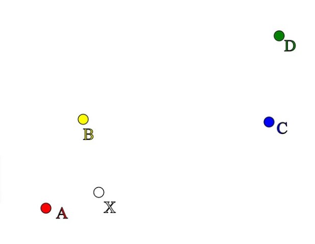
We will use these points to illustrate the basics of interpolation using Leapfrog’s FastRBF™ tool. The grade samples have the values:
| Point | A | B | C | D |
| Grade | 10 | 7 | 1 | 3 |
FastRBF™ combines the known grade values at A, B, C, and D to produce an estimate at X. The simplest approach is to take the average value of all the known grades and then use this average value for the estimate at X. If we use this method, then the estimate will be the same no matter where we look. So when we look at a point close to the high value at A, the estimate is the same as if we look at a point close to the low value at D.
Clearly this is not ideal, it seems reasonable to assume that the estimated value should be more heavily influenced by values from samples that are closer than by those that are further away. To do this Leapfrog uses a function called an interpolant. This interpolant defines how much importance to give each sample based on its distance from the point X.
Interpolants
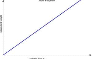
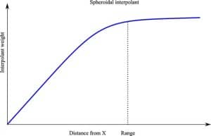
There are two commonly used interpolants in Leapfrog: the linear interpolant and the spheroidal interpolant. These are similar to the linear and spherical variogram models which are used by other packages to perform kriging. Both are illustrated below:
The interpolant is used to assign a weighting to each grade A, B, C and D based on the distance of the sample from the point X at which we want to compute an estimate. Samples that are assigned lower weightings by the interpolant will have a stronger effect on the value of the estimate than those that are given larger values.
The linear interpolant simply assumes that data closer to the point at which you wish to compute an estimate is more important than data that is far away. This importance is inversely proportional to distance from the estimation point X. If we plot the data points on the interpolant graph is looks like this:
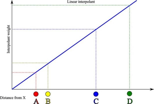
The high grades of 10 and 7 at points A and B will have the most effect on the estimated value computed at X as they are closer. These points are given a lower weighting than C and D. If we use the linear interpolant in Leapfrog to compute the estimated value at X, Leapfrog calculates a value of 7.84 which is indeed between the high grade values. The low grades 3 and 1 at points C and D have a much weaker effect on the estimate as the interpolant gives them a much higher weighting. As a result, the estimated value is closer the nearby high grade values. Overall estimates produced using the linear interpolant will strongly reflect values at nearby points.
The spheroidal interpolant is a bit different. Notice that the spheroidal interpolant flattens out when the distance from X is greater than a defined distance. This distance is known as the range. Sample locations that are within the range are assigned an importance based on their distance from X in the same way as in the linear interpolant method. Samples that are further from X than the range will be assigned roughly the same importance, i.e. these points will have roughly the same influence on the estimate no matter how far away they are. If we plot the data points from the interpolant on a graph it looks like this:
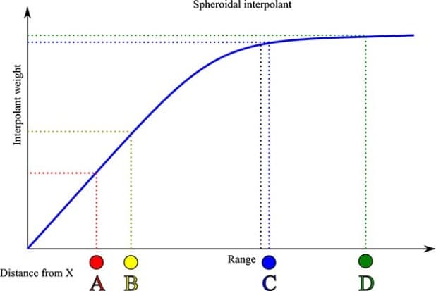
The first part of the graph where points A and B are looks the same as before, i.e. A and B are both close to X so they are given a low weighting and thus will have the largest effect on the estimated value. However the distance of both C and D from X is larger than the range. This puts them on the flat part of the interpolant curve, and means that both are given roughly the same weighting, i.e. C and D have roughly the same influence on the estimate. D has slightly less influence than C but this difference is small. However, as the interpolant weighting curve flattens out when compared to the graph of the linear interpolant, the low grade value at D will have more of an influence on our estimated value than before, i.e. the estimated value should be smaller. This is indeed what happens, as when Leapfrog is using the spheroidal interpolant, for these values it produces an estimate of 6.95 – lower than the estimate of 7.84 produced by the linear interpolant.
This means that if we compute an estimate at a point which is separated from the points A, B, C and D by more than the range, the estimate will all be given a value approximately equal to the average of values of the samples.
In contrast, when using the linear interpolant, the estimate is always influenced most by the closest sample points. This is still the case even when all the samples are a great distance from the estimation point. If this behaviour is not desired, the spheroidal interpolant can limit this effect with the range setting.
Leapfrog’s application of interpolation
Interpolation isn’t a new technique; many other software suites use a method of interpolation known as kriging. The difference with Leapfrog’s FastRBF™ is that it dramatically speeds up the interpolation process, making it much faster than anything else currently available. This tool is used extensively throughout the Leapfrog software suite to accelerate the geological modelling process. The speed with which geological models can be produced enables users to produce alternative models and look at alternative hypotheses which all help to improve decision making and reduce risk.
We’re continually improving performance and have recently developed a new FastRBF™ engine for use in our latest release, Leapfrog Geo. Leapfrog Geo’s new intuitive workflow approach to geological modelling builds on and leverages our experience so far. With Leapfrog you can expect extremely fast implicit modelling for more realistic, sophisticated and robust evaluation.