


Introduction
Multilayer cover systems are often placed over mine wastes to support the growth of native plant species. The cover system must be designed to provide sufficient water and nutrients for the vegetation while protecting the root zone from upwards migrating dissolved solutes originating in the underlying waste. The goal of the design is to minimize the total cover depth while ensuring that the vegetation can be properly supported. The land-climate-interaction boundary condition in SEEP/W is best suited for simulation of the water dynamics in these types of systems because it considers precipitation, snowmelt, evaporation, runoff, and root water uptake occurring below the ground surface.
The objective of this example is to illustrate the application of the land-climate interaction (LCI) boundary condition to simulate the measured hydraulic response in an engineered soil cover and underlying waste material subject to measured climate variability. The cover system overlies a portion of a large saline–sodic overburden dump at the Syncrude Mine site north of Fort McMurray, Alberta. Huang et al. (2015) explored the soil water dynamics of six different cover systems supporting various qualities of vegetation. The performance of only one of those six cover configuration is simulated as part of this example. The journal publication by Huang et al. (2015) forms the basis of much of the information presented in this example file.
A secondary objective of this example is to illustrate the graphs that are available in SEEP/W to assist with interpretation; namely the graphs that assist with closing the water balance, tracking volumes of water stored within the cover, and checking for convergence problems via the water balance error.
Land-Climate Interaction Boundary Condition
The LCI boundary condition comprises two components: one for calculating the net infiltration at the ground surface and another for calculating the root water uptake (RWU) within the soil profile. The mass conservation statement at the ground surface can be written as:
where superscripts on the water fluxes (𝑞) indicate rainfall (𝑃) , snow melt (𝑀), infiltration (𝐼), evaporation (𝐸) and runoff (𝑅) and 𝛼 is the slope angle. The evaporation and runoff fluxes are negative; that is, out of the domain. The infiltration is deemed the residual of the mass balance equation and therefore forms the boundary condition of the water transfer equation. Transpiration does not appear in Equation 1 because root water uptake occurs below the ground surface. Precipitation and snow melt fluxes are incident upon a horizontal surface and must therefore be multiplied by the cosine of the slope angle.
The applied infiltration flux might cause ponding, in which case the pore-water pressure could be set to zero and the time step resolved. Runoff would then be calculated at the end of a time step (boundary review) as:
Evaporation and transpiration can occur unabated if water is fully available and chemical stresses are absent. The combined water flux is referred to as the potential evapotranspiration(𝑃𝐸𝑇). The portion of the potential evapotranspiration that is potential evaporation is:
and the portion that is potential transpiration flux is:
where 𝑆𝐶𝐹 is the Soil Cover Fraction that varies from zero to one for bare ground to full coverage conditions, respectively.
Evapotranspiration Methods
There are various empirical and theoretically based expressions for calculating potential evapotranspiration. The theory based combination equations, which comprise both a radiation and a mixing/aridity component, include the well-known Penman-Monteith and Penman-Wilson equations, both of which are available to the LCI boundary condition in SEEP/W.
Penman-Monteith
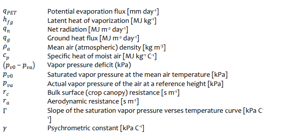
The Penman-Monteith equation for calculating potential evapotranspiration is well accepted in 𝑞𝑃𝐸𝑇 the soil science and agronomy fields and is the recommended procedure of the FAO (Allen et al.,1998):
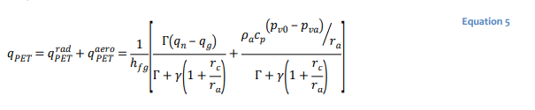
where
The radiation term considers the difference between the net radiation flux and the ground heat flux while the aerodynamic term considers the vapor pressure deficit. The ground heat flux is, however, considered to be zero. The aerodynamic resistance 𝑟𝑎 controls the transfer of water vapor from the evaporating surface into the air above the canopy and is given by (Allen et al., 1998):
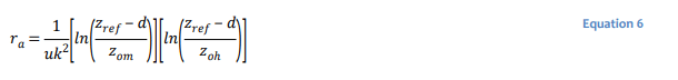
where
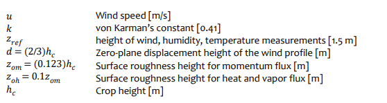
The zero-plane displacement height (𝑑) and surface roughness parameter for momentum (𝑧𝑜𝑚 ) are generally assumed to be some fraction of the vegetation height (Monteith, 1981; Brutsaert, 1975). The roughness parameter for heat and water vapor is assumed to be a fraction of the roughness parameter for momentum (Allen et al., 1998; Dingman, 2003; Saito and Simunek, 2006).
The crop canopy resistance 𝑟𝑐 controls the transfer of water vapor through the transpiring crop and can be estimated by (Allen et al., 1998):
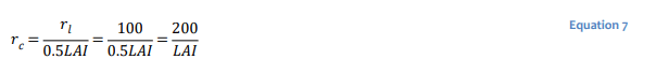
where 𝑟𝑙 is bulk stomatal resistance of the well-illuminated leaf [s m-1]. The 𝐿𝐴𝐼 cannot be zero (bare ground) in Equation 7, so the 𝐿𝐶𝐼 is constrained to a minimum value of 0.1.
Penman-Wilson
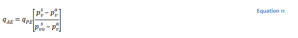
Penman-Wilson developed an expression to calculate the actual evaporation from a bare ground surface ![]() . The actual evaporation from a vegetated surface is calculated as:
. The actual evaporation from a vegetated surface is calculated as:
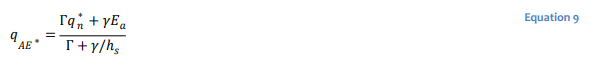
where the aridity is given as:
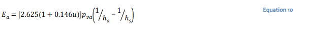
and
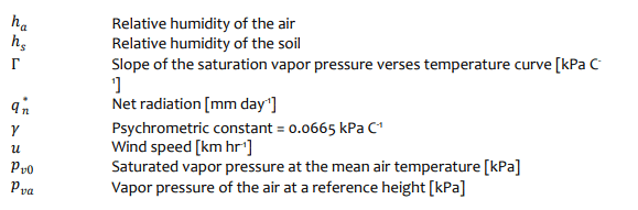
The calculation of the relative humidity at the ground surface requires temperature and matric suction. Temperature at the ground surface is known if a heat transfer simulation is completed. Otherwise the ground temperature is assumed equal to the air temperature.
User Defined
The potential evapotranspiration could be measured on-site or estimated using a variety of methods including the Penman, Thornthwaite, or Monteith methods. The portion of the potential evapotranspiration that is potential evaporation (𝑃𝐸) is then calculated according to Equation 3. The potential evaporation must also be reduced to account for water availability within the soil. Wilson et al. (1997) proposed the following relationship between the actual and potential evaporation fluxes:
Root Water Uptake


where 𝛼𝑟𝑤 and 𝛼𝑟𝑠 are the reduction factors due to water and salinity stresses, respectively. The term 𝛼𝑟𝑤 is defined by a plant limiting function. The LCI boundary condition in SEEP/W does not accommodate salinity stresses. A more complete understanding of the root water uptake boundary condition can be obtained by reviewing the associated example files.
Study Site
The study site, referred to as the South Bison Hills (SBH), is located within the oil sands region of Northern Alberta. Saline-sodic shales were removed in order to extract the underlying oil sands. Large overburden dumps of shale were contoured and reclaimed using multilayer covers comprising a mixture of salvaged peat and glacial mineral soil placed over a thicker horizon of salvaged glacial mineral soil (Boese, 2003; Dobchuk et al., 2012). Three covers, referred to as D1, D2, and D3, were constructed on the north facing slope, and a fourth cover was constructed on the plateau. The hydraulic response of the D2 soil cover system is being considered in this study. The thermal response of the D2 soil cover system was explored in another example. The D2 cover comprises 15 cm of a peat-mineral mix overlying 22 cm of a till/secondary cover material.
Weather stations are located on the plateau and north facing slope. Weather data collected at these locations include precipitation, temperature, wind speed, wind direction and relative humidity. Net radiation is also measured at the weather station on the plateau (Boese, 2003; O’Kane Consultants Ltd., 2013). Carey (2008, 2001) measured surface water and energy exchange using the eddy covariance techniques. Soil monitoring stations were installed within each cover system. Temperature sensors were installed at depths 5, 10, 20, 25, 32, 42, and 80 cm. Volumetric water content and matric suction sensors were installed at depths 5, 10, 20, 30, 40, 50, 65, and 80 cm (O’Kane Consultants Ltd., 2012).
Carey (2008 and 2011) found that from 2003 to 2009, the peak leaf area index (LAI) increased from 0.5 to 2.8, and the growing season partitioning of energy showed a strong increase in the fraction of net radiation partitioned into latent heat. As is shown in the associated example simulating the thermal response, a steady collapse in the yearly difference between the maximum and minimum ground temperatures, along with a dampening of diurnal variability, occurs from mid-1999 to the end of 2003 show. The changes in the measured thermal response correlate to the development of the invasive weed species, evolution of the aspen stand, and the development of the Litter Fermented Humus (LFH) organic layer and grass thatch.
The hydraulic properties of the soil covers also evolved as a result of biological processes, freeze-thaw and wet-dry cycling, settlement of the cover materials and underlying waste, vegetation rooting and other physical processes. Macropores and fractures developed within the predominantly clay soils. These structures had a control on the hydrogeological response of the covers during the spring freshet. Kelln et al. (2007) used hydrometric data to determine that snowmelt water initially infiltrated into the macrospores where it froze. The fresh water was subsequently released from the macropores during thaw, descending through the soil cover and mixing with the antecedent water within the soil matrix. The mixed water eventually perched on the
lower conductivity shale and flowed downslope.
Kelln et al. (2008) used numerical simulations to evaluate the performance of the covers. The modeling demonstrated a cover thickness greater than 50 cm was necessary to sustain tree growth while creating a sufficient buffer between the high-salinity pore water near the cover-shale interface and root zone.
Numerical Simulation
There are two commonly applied options for simulating water flow in system with structures such as fractures and macropores: an equivalent porous media model in which one set of hydraulic properties is used or a dual porosity model. Both approaches are valid representations of the system. Kelln et al. (2009) used the former approach while Huang et al. (2015) used the later approach. SEEP/W is a single porosity finite element formulation; consequently, the materials were represented as an equivalent porous media.
The water dynamics in the cover system and underlying waste are being simulated using a 1D finite element formulation (see GeoStudio file). Downslope flow of water along the shale interface – that is, interflow – following the thaw and release of water in the macropores cannot be accommodated in the analysis. Huang et al. (2015) noted that a 1D model adequately represents the soil water dynamics within the cover despite this deficiency because the interflow volumes are small and the lateral flow occurs over a short duration.
The entire 5 year period between 2009 and 2013 is being simulated in the example. In contrast, Huang et al. (2015) modeled only the days of the year during which the ground was unfrozen at all measurement locations. The measured water content profiles just prior to freeze-up were used to define the initial conditions in the spring of the subsequent year. Huang et al. (2015) also had to calculate total snowpack volumes and convert this into a liquid water flux that was applied as a boundary condition each spring. This modeling methodology could have been accomplished in SEEP/W using spatial functions of pressure head to define the initial condition uniquely in each year.
Alternatively, the parent-child functionality could have been used if the simulated results at the end of each analysis year were used to define the initial condition of the subsequent year. The advantages of simulating the entire 5 year period, despite the greater simulation times, are that it simplifies the analysis definition and allows for water redistribution during the winter months. More importantly, the land-climate boundary condition calculates the snow melt flux in accordance with the user defined snow depth-time function, which could be measured or estimated from the precipitation record.
Soil Profile
Field monitoring data indicated that the overburden shale beneath the relatively thin D2 cover is subject to seasonal wetting and drying cycles. As such, the shale must be included in the numerical simulation. The simulated one-dimensional soil profile consists of 15 cm of a peat-till mineral mixture, which overlies 22 cm of a secondary, till cover material, and 9.63 m of the underlying overburden shale material. The shale thickness, although arbitrary, was great enough to ensure that the hydraulic response was negligible near the bottom boundary.
Hydraulic Properties
Huang et al. (2015) used an optimizations scheme to obtain the van Genuchten (1980) material properties shown in Table 1. These properties provided the best calibration between the measured and simulated response of the dual-porosity formulation for the D2 cover. The average (bulk) hydraulic conductivity values, which theoretically only represent the mobile phase (i.e. macropores and fractures), were measured by Meiers et al. (2011).
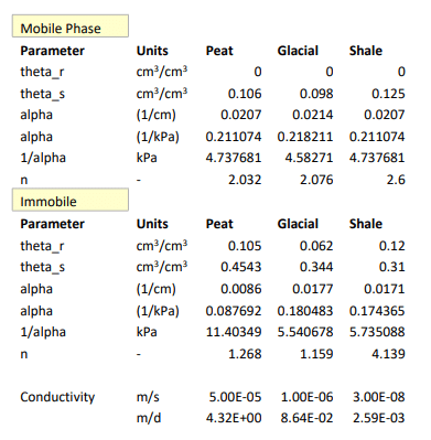
Table 1. Calibrated material properties for the mobile and immobile phases used by Huang et al. (2015).
SEEP/W’s formulation requires that each unit be represented by a single set of hydraulic properties. In addition, the optimized parameters shown in Table 1 can only be used as a guide given that the basis for the estimation was a dual-porosity formulation. As a first step, the volumetric and hydraulic conductivity functions for the immobile and mobile phases were estimated using the van Genuchten properties shown in Table 1. The conductivity functions for mobile phases were anchored at the (bulk) average hydraulic conductivity (Table 1; Meiers et al., 2011) while those of the immobile phase were either anchored at the same value or shifted down one or two orders of magnitude.
Kelln et al. (2009) used composite hydraulic functions to represent the glacial clay-rich soil overlying the shale. In a similar manner, a composite hydraulic conductivity function was developed from the conductivity functions of the immobile and mobile phases. The saturated hydraulic conductivity values of the immobile and mobile phases were 8.64E-03 m/d and 8.64E-02 m/d (Table 1), respectively. A composite hydraulic conductivity function was created for the glacial soil by transitioning from the mobile to the immobile function at the intersection point. Kelln et al. (2009) also used a composite volumetric water content function defined as the summation of the two individual functions; however, in this study the behavior of the glacial soil was assumed adequately represented by the function for the immobile phase.
Both the peat and shale were represented by the hydraulic functions for the immobile phase. The corresponding hydraulic conductivity functions were anchored at the at the (bulk) average hydraulic conductivity values shown in Table 1. A unique material model was created to represent the shale in the lower part of the profile for reasons that will be explored subsequently. The material property definitions can be examined in the associated GeoStudio project file.
Initial and Boundary Conditions
The initial condition for the transient analysis was defined using the activation pore-water pressure in the material definition. The negative activation pore-water pressures for each material were selected to approximate the measured volumetric water contents at the end of fall 2008.
A land-climate-interaction boundary condition was applied to the top of the domain and a unit hydraulic gradient to the bottom of the domain. The land-climate-interaction boundary condition comprises climate and vegetation data defined over a 5 year period between 2009 and 2013 (i.e. duration of 1826 days). The climate and vegetation function definitions can be examined in the associated GeoStudio project file. Note that the snow depth-time function was measured on the top of the 30D overburden dump. It is also worth noting that Huang et al. (2015) estimated rainfall interception in accordance with the 𝐿𝐴𝐼, which is then subtracted from the measured precipitation to calculated the flux on the ground surface (beneath the canopy). Interception was not accounted for in this example.
Potential evapotranspiration was calculated using the Penman-Monteith equation (Equation 5). The potential evapotranspiration is partitioned into potential evaporation and potential transpiration using the soil cover fraction (Equation 3 and Equation 4). Ritchie (1972) proposed the following equation, based on interception of the solar radiation by canopy, for apportioning the potential evapotranspiration into potential evaporation and transpiration fluxes:
where 𝐿𝐴𝐼 is the leaf area index and 𝑘 is a constant governing the radiation extinction by the canopy as a function of sun angle, the distribution of plants, and the arrangement of leaves. The 𝑆𝐶𝐹 function was estimating using 𝑘 equal to 0.5 and an 𝐿𝐴𝐼 time function defined between Day 135 and 290 of every year (Huang et al., 2015). A maximum 𝐿𝐴𝐼 = 2.0 was reached between Day 195 and 225.
The normalized water uptake distribution is required to calculate the maximum potential transpiration flux at any depth (Equation 12). This value is calculated by the solver from the user entered normalized root density function. The input normalized root density function was based on field measurements by Shurniak (2003), which suggested that the bulk of the root mass is contained within the peat-mineral mix, decreasing logarithmically through the glacial soil. Correspondingly, the root depth-time function extends the roots to the till-shale interface. Equation 13 requires the
reduction factors due to water stresses 𝛼𝑟𝑤. Huang et al. (2015) decreased 𝛼𝑟𝑤 from 1.0 to 0.0 between matric suctions of 500 kPa and 1900 kPa.
Results and Discussion
Water Storage
Figure 1 through Figure 5 show the simulated and measured volumetric water contents at depths of 5 cm, 10 cm, 32 cm, 42 cm, and 80 cm. Verification of the results by way of a comparison between measured and simulated volumetric water contents is not ideal because of the sensitivity of the measurement to changes in texture and density. Having stated this, the simulated volumetric water contents generally reflect the overall measured response at all depths and can therefore be used to interpret the response of the physical system.
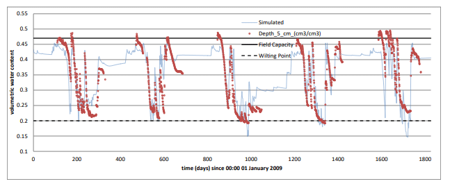
Figure 1. Simulated versus measured volumetric water content-time history at 5 cm depth (Peat-mineral mixture).
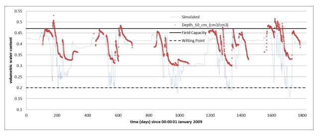
Figure 2. Simulated versus measured volumetric water content-time history at 10 cm depth (Peat-mineral mixture).
Simulated water contents in the peat track well with the measured response, which correlated strongly with snowmelt, rainfall, and prolonged evapotranspiration throughout the cover. The simulated response at 10 cm is nearly identical to that at 5 cm, which is in closer agreement with the measured response. Measured water contents at 10 cm, however, do not approach the wilting volumetric water content of 0.20 at any point during the 5 year period, which is rather remarkable given the close proximity to the overlying sensor, the proximity to the ground surface, and the root density at this depth. Shurniak (2003) measured in situ volumetric water content functions in the covers and observed a sharp change in behavior at 7.5 cm depth. The ‘deep’ peat layer was proposed to be a mixture of peat and till, which would explain the increased water retention capacity during the dry periods.
Simulated and measured water contents in the glacial soil generally have more muted responses to climate conditions (Figure 3). In comparison to the thicker cover systems, however, the 32 cm sensor demonstrated persistent changes in water content. The measured volumetric water content at 20 cm was also included on Figure 3 to illustrate that the simulated response reflects the overall measured response rather well despite the heterogeneities.
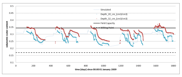
Figure 3. Simulated versus measured volumetric water content-time history at 32 cm depth (Glacial soil).
Volumetric water content changes are also occurring at the top of the shale (Figure 4). A close inspection of the measured response in the shale reveals a time history that tracks, in a relative sense, more closely with the response in the glacial soil (Figure 3). Persistent changes in the volumetric water content were only observed in the upper portion of the shale in the thinnest D2 cover and at one other location on the plateau. As noted by Huang et al. (2015), the measured minimum water content at 42 cm depth is lower than the wilting point (~0.20) of the shale because of the presence of a somewhat coarser material at this location and/or a greater percentage of root biomass penetrating the shale. Huang et al. (2015) noted that the shale overburden can be
particularly heterogeneous, ranging from clay shale to lean oil sands. The D2 cover is the only location at which the water balance within the cover is affected appreciably by water content changes in the shale. The measured and simulated responses are highly muted deeper in the shale at 80 cm (Figure 5).
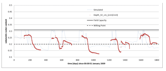
Figure 4. Simulated versus measured volumetric water content-time history at 42 cm depth (Shale).
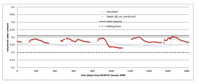
Figure 5. Simulated versus measured volumetric water content-time history at 80 cm depth (Shale).
An alternative means of considering storage changes is to compare the simulated and measured water storage within the cover (Figure 6). The measured values were obtained by averaging the volumetric water contents measured in each layer of the cover and multiplying by the thickness of the unit, assuming 1 unit in the out-of-plane direction. There was no attempt to associate each senor with a characteristic length given the variability within each layer, which may account for part of the discrepancy with the measured storages presented by Huang et al. (2015). Simulated values of stored water volumes within each layer were obtained via Draw – Graph (refer to the associated GSZ project file), divided by the unit area of the column, and converted into millimetres. The graph is generated by selecting a subdomain – that is, a group of elements within the larger domain – that comprises the entire soil cover.
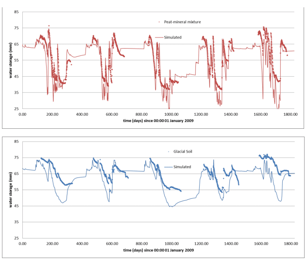
Figure 6. Comparison of the simulated and measured water storages in the peat-mineral mixture and glacial soil.
The overall losses or gains in water are simulated very well despite the discrepancies in the instantaneous values. For example, the peat-mineral and glacial soil were particularly dry in the fall of 2011, at around Day 1050. Huang et al. (2015) note that part of the discrepancy may be related to the presence of leaf fibre humus and mulch on the ground surface that acted to suppress soil evaporation. Incidentally, the presence of this material had a significant effect on the thermal response within the domain because it acted as an insulating unit (refer to the associated example file).
The reasonable match suggests that the material characterization, climate data definition, and root water uptake models are adequate to simulate daily water balance for the cover systems. The analysis duration could therefore be increased and sensitivity analyses completed to assess the ability of the cover to support vegetation under various climate scenarios as was done by Huang et al. (2015). Huang et al. (2015), for example, compiled the results of the sensitivity analyses in a manner that allowed for the realization that the thinner cover productivity is affected by dry year cycles in which the maximum evapotranspiration would actually limit the leaf area index, which would in turn further restrict transpiration and therefore plant productivity. Huang et al. (2015) also demonstrated that the incremental increases in cover thickness do not produce proportional increases in actual transpiration. There was little incremental increase in the median actual transpiration once the cover thickness exceeded 100 cm.
Water Balance Components and Deep Percolation
Figure 7 shows the water balance components for the D2 cover in cumulative water volumes (m3). End-of-simulation volumes were used to calculate yearly average values. For discussion purposes, the cumulative water volumes were normalized by the cross-sectional area of the column (1.0 m2), converted into units of millimetres (i.e. m3/ m2 x 1000 mm/m), and divided by 5 (years) to obtain the year average. For example, the simulated end-of-simulation rainfall was 1.43 m3, which amounts to an average yearly rainfall of 286 mm. The simulated average yearly snowmelt was 35 mm, for a total
precipitation of 321 mm. The simulated rainfall (286 mm) is exactly equal to the 5-year average calculated from the input precipitation function because snowfall as water equivalent was not included in the data. It is worth noting, however, that the input function could have included snowfall as a water equivalent, in which case the 5-year average from the function would have been 367 mm, but the simulated rainfall would have remained at 286 mm. Precipitation is not tracked as rainfall when the average air temperature is below 0 degrees Celsius. In addition, the total simulated rainfall and snowmelt of 321 mm is less than 367 mm because snowmelt is controlled by the snow depth function, which accounts for ablation and other factors.
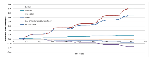
Figure 7. Water balance components for the D2 Cover.
The simulated average potential evapotranspiration was 350 mm (not shown on Figure 7) while the average actual evapotranspiration, calculated as the summation of the average evaporation and average root water uptake, was 265 mm. Huang et al. (2015) reported an average potential evapotranspiration of 495.8 mm. As noted previously, the crop canopy resistance 𝑟𝑐 approaches infinity as the 𝐿𝐴𝐼 approaches zero in Equation 5; consequently, the potential evapotranspiration, and therefore evaporation and transpiration (i.e. root water uptake), is zero during the spring and late fall when the 𝐿𝐴𝐼 is zero (refer to the associated example file). The ‘real’ average potential evapotranspiration has to be calculated using the Penman-Wilson method (i.e. Penman method). The Penman potential evapotranspiration was calculated as 593 mm (note: this value was obtained by changing the Evapotranspiration method in the boundary condition to ‘Penman-Wilson’). The average ratio of yearly actual evapotranspiration to potential evapotranspiration was 45% (265/593).
The average ratio of yearly actual evapotranspiration to total precipitation was 83% (262/315). Twenty-six percent (26%) of the actual evapotranspiration of 265 mm was transferred by actual evaporation (69 mm). Huang et al. (2015), using a LAI of 3.5, simulated actual evapotranspiration plus interception that accounted for 92% of the precipitation, of which 14 to 16% was by actual evaporation. This value was lower than SEEP/W because a portion of the precipitation was removed a priori to account for interception. Black et al. (1996) studied a boreal aspen forest with an LAI of 3.3 and observed that 88% of the precipitation was removed by evapotranspiration and interception evaporation. Only 5% of the evapotranspiration was transferred to the atmosphere by actual evaporation. Huang et al. (2015) suggested that the presence of mulch on the cover, which was not accounted for in the simulations, likely suppressed the evaporation flux.
Huang et al. (2015) note that the total run-off measured at four weirs at various locations averaged 34 mm from 2003 to 2012 and varied from 18.5 to 47 mm. The SEEP/W analysis reported a runoff of -0.15m3, which is about 30 mm when converted to millimeters and averaged over the 5 years. The simulated value is slightly lower than the measured; however, the measured value likely includes interflow along the till-shale interface. In general, the magnitudes of the simulated water balance components for the D2 cover are consistent with the simulated and measured values presented by Huang et al. (2015).
The simulated deep percolation (-0.13 m3; Figure 8), which when converted into millimetres and averaged over 5 years, is approximately 30 mm. Deep percolation past the base of the cover predominantly occurs during snowmelt when the vegetation is inactive. In fact, almost all of the precipitation is utilized by the vegetation during the growing season.
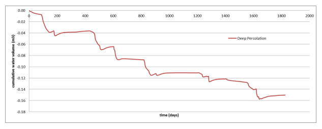
Figure 8. Cumulative water volume past the base of the cover.
Huang et al. (2015) completed a rigorous sensitivity study involving 60 years of climate data, various cover thicknesses, and various leaf area index values and observed this to be true regardless of cover thickness. The measured snowpack volume varied from 49 to 215 mm water equivalent, with an average of 116 mm. The difference between the volumetric water contents at field capacity (0.37) and the wilting point (0.18) for the glacial till is 0.19. The till would therefore have to be 610 mm (i.e. 116 mm/0.19) thick to store the snow melt for subsequent uptake by the vegetation. The 22 cm of till in the D2 cover is obviously not adequate from this perspective; however, as noted by Huang et al. (2015) a potential downside of thick covers is a loss of water released to adjacent wetlands that are required to support the ecosystem.
Mass Balance Error
Non-convergence at any time step of a transient finite element analysis can manifest in an inequality between the rate of change in the mass of water stored within the domain and the rate at which water enters and leaves the domain. The difference between the cumulative change in mass of water within the domain and the cumulative mass that leaves or enters the domain provides a measure of the error. A relative error could be calculated by dividing the absolute error by the maximum of the two values. The mass balance error and its components can be plotted for the entire domain or portion of the domain; that is, a subdomain. Figure 9 was generated for the cover materials (refer to the associated file). The cumulative change in mass within the domain is generally commensurate with the cumulative change at the boundaries, including root water uptake. The mass balance error is therefore negligible after five years.
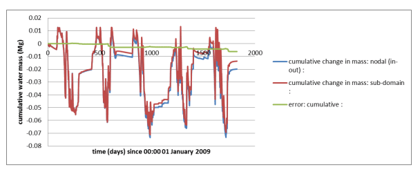
Figure 9. Mass balance error.
Summary and Conclusion
This example file illustrates how the land-climate-interaction boundary condition can be used to simulate the hydraulic response in an engineered soil cover subject to measured climate variability. Interpretation of a land-climate-interaction analysis is done primarily by way of an exploration of the stored water volumes, deep percolation (i.e. past the base of the cover), and graphs of the water balance components. The water balance components lend insight into how much of the precipitation and snowmelt infiltrates, how much of the infiltrating water is evaporated and transpired, and therefore what portion percolates deeper into the soil profile. Absolute and relative water balance error graphs are used to ensure that convergence is acceptable at all points in the simulated time history.
The simulated SEEP/W results reflected the measured patterns for the published case study, indicating that the characterizations of the hydraulic properties, geometry, and boundary conditions adequately represent the physical reality. This example considered a single cover system and 5 years of climate data. Optimizing the cover design would require additional simulations to explore various cover thicknesses, vegetation scenarios, and climate variability. The objective of the sensitivity study would be to understand the mechanisms underlying changes in soil water storage and transpiration arising as result of increasing cover thickness. The cover could then be designed with a thickness that supports vegetation growth and release of water to the wetlands while slowing the upwards migration of salts (Huang et al, 2015).
References
Allen, R.G., Pereira, Luis S., Raes, D., Smith, M. 1998. Crop evapotranspiration – Guidelines for computing crop water requirements – FAO Irrigation and drainage paper 56. Food and Agriculture Organization of the United Nations.
Feddes, R.A., Hoff, H., Bruen, M., Dawson, T. de Rosnay, P., Dirmeyer, P., Jackson, R.B., Kabat, P., Kleidon, A., Lilly, A., Pitman, A.J. 2001. Modeling root water uptake in hydrological and climate models. Bulletin of the Americal Meteorological Society. Volume 82 (12): 2797 – 2809.
Huang MB, Barbour SL, Elshorbagy A, Zettl JD, Si BC. 2011. Water availability and forest growth in coarse textured soils. Canadian Journal of Soil Science 91: 199–210.
Huang, M., Barbour, S.L. Carey, S.K. 2015. The impact of reclamation cover depth on the performance of reclaimed shale overburden at an oil sands mine in Northern Alberta, Canada. Hydrological Processes: 29: 2840-2854.
Kelln C.J. 2008. The effects of meso-scale topography on the performance of engineered soil covers. Ph.D. Dissertation, University of Saskatchewan, Saskatoon, SK.
Kelln C.J., Barbour S.L., Qualizza C.V. 2007. Comparison of tree growth statistics with moisture and salt dynamics for reclamation covers over saline-saodic overburden. Proc., Canadian Land Reclamation Association Symp., Halifax, North Scotia, Canada.
Kelln C.J., Barbour S.L., Qualizza C.V. 2008. Controls on the Spatial Distribution of Soil Moisture and Salt Transport in a Sloping Reclamation Cover. Canadian Geotechnical Journal 45(3): March, 10.1139/T07-099, 351–366.
Kelln C.J., Barbour S.L., Qualizza C. 2009. Fracture-dominated subsurface flow and transport in a sloping reclamation cover. Vadose Zone Journal 8: 96–107.
Meiers G., Barbour S.L., Qualizza C., Dobchuk B. 2011. Evolution of the hydraulic conductivity of reclamation covers over sodic/saline mining overburden. Journal of Geotechnical and Geoenvironmental Engineering 137(1): 968–976.
Shurniak R.E. 2003. Predictive modeling of moisture movement within soil cover system for Saline/Sodic overburden piles. M. Sc. Thesis.
University of Saskatchewan, Saskatoon, Saskatchewan, Canada.
Wilson, G.W., Fredlund D.G., and Barbour S.L. 1997. The effect of soil suction on evaporative fluxes from soil surfaces. Canadian Geotechnical Journal. Volume 34: 145-155.