Introduction & What’s New in Target for ArcGIS Pro 2.4

Easily import and visualise, then share your knowledge and make discoveries faster using the ArcGIS Pro tools you’re familiar with.

An introduction of Target for ArcGIS Pro while highlighting all the newest features available in the latest release. Discover how to unlock more ways to visualise, share and understand your drillhole and subsurface data:

Target for ArcGIS Pro 2.4 introduces new features that allow you to import and view Geosoft voxels and draw Geologic interpretations.

• Rapidly import Geosoft voxels into Target for ArcGIS Pro as NetCDF format files
• Utilise ArcGIS Pro’s native NetCDF functionalities to display, filter and slice voxels for better interpretation
• Create drawings on 2D cross sections or in 3D scenes to capture your understanding of geology and subsurface relationships.
• Easily manage and publish interpretations using Esri’s ArcGIS online

Overview

Video Transcript

1
00:00:01,640 –> 00:00:04,010
<v Narrator>Hello, welcome to Seequent’s webinar,</v>

2
00:00:04,010 –> 00:00:09,010
on the newest release of Target for ArcGIS Pro version 2.4.

3
00:00:09,320 –> 00:00:11,060
My name is Comedic Hallett,

4
00:00:11,060 –> 00:00:14,100
and I’d like to thank you today for joining in.

5
00:00:14,100 –> 00:00:15,950
Well people are logging on here.

6
00:00:15,950 –> 00:00:17,890
I’ll just go ahead and introduce myself.

7
00:00:17,890 –> 00:00:19,127
My name is Kate Kaled

8
00:00:19,127 –> 00:00:21,570
I’m a geophysicist here at Seequent

9
00:00:21,570 –> 00:00:24,890
based in our north America branch in Toronto.

10
00:00:24,890 –> 00:00:27,474
And here at Seequent, I work largely within

11
00:00:27,474 –> 00:00:31,460
our technical team, and I collaborate often

12
00:00:31,460 –> 00:00:33,780
with our other business units as well.

13
00:00:33,780 –> 00:00:37,410
And we work together to find solutions

14
00:00:37,410 –> 00:00:40,053
for two sense professionals, such as yourselves.

15
00:00:40,900 –> 00:00:44,480
Okay, so with introductions out of the way,

16
00:00:44,480 –> 00:00:47,290
let’s dive into the agenda.

17
00:00:47,290 –> 00:00:49,840
A bit of webinar logistics.

18
00:00:49,840 –> 00:00:52,876
If you have any questions, please type them into the chat.

19
00:00:52,876 –> 00:00:56,630
And we’ll be sure to get back to you after the webinar,

20
00:00:56,630 –> 00:00:58,580
we’ll be reaching out to you via email.

21
00:01:00,700 –> 00:01:04,000
So today we’ll be going over a general overview

22
00:01:04,000 –> 00:01:07,810
of Target for ArcGIS Pro and how it can benefit

23
00:01:07,810 –> 00:01:11,253
your exploration and project workflows.

24
00:01:11,253 –> 00:01:14,220
We’re going to keep it fairly high level.

25
00:01:14,220 –> 00:01:16,280
I’m going to give you some of the highlights

26
00:01:16,280 –> 00:01:18,970
of the key features in the software.

27
00:01:18,970 –> 00:01:20,534
And for those of you who are new to

28
00:01:20,534 –> 00:01:22,250
Target for ArcGIS Pro,

29
00:01:22,250 –> 00:01:25,400
I’m going to go over some of the main functionalities,

30
00:01:25,400 –> 00:01:28,680
like Geohole import, Geohole visualization,

31
00:01:28,680 –> 00:01:30,680
cross section preshift,

32
00:01:30,680 –> 00:01:34,400
importing files like dual up grids,

33
00:01:34,400 –> 00:01:38,820
and mesh files, and how to create strip logs,

34
00:01:38,820 –> 00:01:39,993
enjoyable planning.

35
00:01:41,960 –> 00:01:43,877
What the main features out of the way,

36
00:01:43,877 –> 00:01:46,780
we’re going to go into the newest features

37
00:01:46,780 –> 00:01:49,397
that have been added to the target product,

38
00:01:49,397 –> 00:01:52,270
ArcGIS pro functionality list.

39
00:01:52,270 –> 00:01:53,990
In this next police,

40
00:01:53,990 –> 00:01:57,790
we’re very excited to introduce two new features,

41
00:01:57,790 –> 00:02:00,493
that allow you to import and visualize

42
00:02:00,493 –> 00:02:05,493
Geosoft voxels and create geologic interpretation.

43
00:02:05,870 –> 00:02:07,867
These are features that have been

44
00:02:07,867 –> 00:02:10,727
more requested by yourselves.

45
00:02:10,727 –> 00:02:12,360
I’m going to give you an in-app

46
00:02:12,360 –> 00:02:13,870
application demonstration of how

47
00:02:13,870 –> 00:02:16,380
to use these two new features,

48
00:02:16,380 –> 00:02:18,795
and I’m also going to show you how you

49
00:02:18,795 –> 00:02:22,910
can take these interpretations,

50
00:02:22,910 –> 00:02:25,010
these geologic interpretations.

51
00:02:25,010 –> 00:02:30,010
And publish them using esri’s ArcGIS online functions.

52
00:02:32,250 –> 00:02:33,963
Okay, let’s get started.

53
00:02:35,730 –> 00:02:37,950
Okay, let’s start with a general overview

54
00:02:37,950 –> 00:02:39,910
of what’s available to you as a charter

55
00:02:39,910 –> 00:02:42,390
for ArcGIS Pro user.

56
00:02:42,390 –> 00:02:44,860
Here we are in the application,

57
00:02:44,860 –> 00:02:47,210
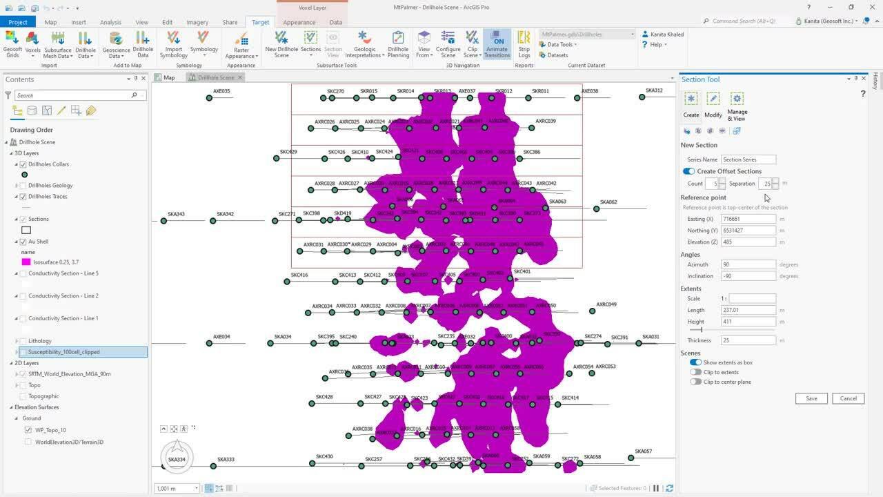
after you download and install the software.

58
00:02:47,210 –> 00:02:50,600
Target for ArcGIS Pro appears as its own ribbon

59
00:02:50,600 –> 00:02:53,790
or menu up here at the top in ArcGIS Pro.

60
00:02:53,790 –> 00:02:55,090
The first thing we’ll probably do

61
00:02:55,090 –> 00:02:57,210
is sign in with your Seequent ID,

62
00:02:57,210 –> 00:03:00,904
so that you can access the functions in the correct ribbon.

63
00:03:00,904 –> 00:03:03,460
On the left hand side of the target ribbon,

64
00:03:03,460 –> 00:03:06,270
you see the import group.

65
00:03:06,270 –> 00:03:08,610
This import group allows me to import

66
00:03:08,610 –> 00:03:12,040
a variety of data types right into my project.

67
00:03:12,040 –> 00:03:15,750
Today we’re looking at a data set, called Mt Palmer,

68
00:03:15,750 –> 00:03:20,063
which is a gold mineralization project in Western Australia.

69
00:03:21,777 –> 00:03:23,230
So the first thing we’ll do,

70
00:03:23,230 –> 00:03:25,960
is look at the Geofill importer.

71
00:03:25,960 –> 00:03:28,720
There are a variety of ways to import drilling data.

72
00:03:28,720 –> 00:03:31,870
The first and quite common way is

73
00:03:31,870 –> 00:03:36,870
by Excel, access or by a TXT or ASCII files.

74
00:03:37,380 –> 00:03:39,710
You can also download your, sorry,

75
00:03:39,710 –> 00:03:43,510
import your drilling data with an ODBC connection.

76
00:03:43,510 –> 00:03:48,510
Either locally on your network or as a TXT file.

77
00:03:50,670 –> 00:03:54,100
And if your organization logs your drilling data

78
00:03:54,100 –> 00:03:57,790
with programs like Wire or Deposit.

79
00:03:57,790 –> 00:04:02,790
You can import data directly in from those programs as well.

80
00:04:03,410 –> 00:04:07,300
Finally, if you have a pre-existing Geosoft target project,

81
00:04:07,300 –> 00:04:09,410
the entire project can be imported

82
00:04:09,410 –> 00:04:11,463
directly into ArcGIS Pro.

83
00:04:12,820 –> 00:04:15,550
And all of the drill hole data that you import in,

84
00:04:15,550 –> 00:04:19,300
will be converted into Geodatabase format,

85
00:04:19,300 –> 00:04:22,700
which is native to esri.

86
00:04:22,700 –> 00:04:25,374
So as an example, when I select drillable data

87
00:04:25,374 –> 00:04:27,310
and then access.

88
00:04:27,310 –> 00:04:31,620
This brings up the Geoprocessing page or important data,

89
00:04:31,620 –> 00:04:35,073
from here, I can select the name of my drill hole data set.

90
00:04:35,073 –> 00:04:40,073
I can assign a spacial reference or coordinate system,

91
00:04:40,889 –> 00:04:42,720
and we can pull those in as our

92
00:04:42,720 –> 00:04:45,029
attributes of the color data, we’ll say color

93
00:04:45,029 –> 00:04:48,112
or survey data, let’s say survey.

94
00:04:48,112 –> 00:04:50,150
And then we also have the option of

95
00:04:50,150 –> 00:04:53,940
organizing our drilling data into interval and point data.

96
00:04:53,940 –> 00:04:58,940
So we can assign, geology and assay data

97
00:04:59,170 –> 00:05:01,720
to be brought in as interval data

98
00:05:01,720 –> 00:05:04,980
and structure as point data.

99
00:05:04,980 –> 00:05:07,343
Which is disparate points down the drill hole.

100
00:05:08,300 –> 00:05:09,920
Once you’ve selected your attributes,

101
00:05:09,920 –> 00:05:10,883
go ahead and press run.

102
00:05:10,883 –> 00:05:13,476
And you have already run this in the back here.

103
00:05:13,476 –> 00:05:15,827
So my data has finished importing.

104
00:05:15,827 –> 00:05:20,160
Now I can go ahead and head into the act two math group,

105
00:05:20,160 –> 00:05:24,820
and bring in my data, so that I can visualize it

106
00:05:24,820 –> 00:05:28,450
onto my 2D map or 3D scene.

107
00:05:28,450 –> 00:05:31,570
So the add data button here allows me to go ahead

108
00:05:31,570 –> 00:05:34,260
and toggle on various attributes,

109
00:05:34,260 –> 00:05:38,943
such as color, traces and my from two data.

110
00:05:41,010 –> 00:05:44,890
And once I do so, that will just load right onto my scene.

111
00:05:44,890 –> 00:05:47,443
And I can zoom in to start visualizing.

112
00:05:56,300 –> 00:05:59,230
From here, I can use the symbology tools

113
00:05:59,230 –> 00:06:04,230
to apply sizes and also offsets to the, to the symbology

114
00:06:07,930 –> 00:06:10,470
Other than drill hole data.

115
00:06:10,470 –> 00:06:13,010
I’m also able to visualize faster data by

116
00:06:13,010 –> 00:06:18,010
importing in red files or Geosoft format grid files

117
00:06:18,290 –> 00:06:21,490
to demonstrate I can select the Geosoft grid tool.

118
00:06:21,490 –> 00:06:24,540
This brings in with your Geoprocessing tool on the right.

119
00:06:24,540 –> 00:06:26,080
And from here you can go ahead and

120
00:06:26,080 –> 00:06:29,520
select the Geosoft grid that you wish to bring in.

121
00:06:29,520 –> 00:06:31,610
I want to bring in my typography.

122
00:06:31,610 –> 00:06:34,410
So I’ll go ahead and look for that in my project folder.

123
00:06:36,010 –> 00:06:36,980
And once I’m ready,

124
00:06:36,980 –> 00:06:40,040
that will get converted into a raster dataset

125
00:06:40,040 –> 00:06:42,593
and important to my Geodatabase.

126
00:06:46,980 –> 00:06:48,560
After it’s finished importing,

127
00:06:48,560 –> 00:06:52,140
it will get displayed on my map scene here,

128
00:06:52,140 –> 00:06:55,390
and we can see that it has retained the original colors

129
00:06:55,390 –> 00:06:57,453
that the geophysicist had applied to it.

130
00:06:59,150 –> 00:07:02,370
And here is an example of a first vertical

131
00:07:02,370 –> 00:07:05,310
derivative grid from a magnetic data site.

132
00:07:05,310 –> 00:07:06,570
Just to show you an example,

133
00:07:06,570 –> 00:07:09,163
the type of data that can be brought in as raster.

134
00:07:11,499 –> 00:07:14,630
One of the advantages of working inside ArcGIS Pro,

135
00:07:14,630 –> 00:07:19,630
is being able to work with multiple maps and PDCs.

136
00:07:19,790 –> 00:07:21,840
So here I have a 2D map open,

137
00:07:21,840 –> 00:07:26,120
but I can easily flip to a 3D scene by selecting

138
00:07:26,120 –> 00:07:29,270
this new drill holes scene option.

139
00:07:29,270 –> 00:07:32,650
So once I select this, I can easily flip over

140
00:07:32,650 –> 00:07:35,933
to a 3D scene just like here.

141
00:07:36,870 –> 00:07:39,210
And here, we have the same typography

142
00:07:39,210 –> 00:07:41,510
and data that we saw on the 2D map,

143
00:07:41,510 –> 00:07:44,270
along with the colors and traces.

144
00:07:44,270 –> 00:07:49,270
And I’ve also clipped my scene to the extent of my,

145
00:07:49,520 –> 00:07:52,730
the spacial extent of my drilling data.

146
00:07:52,730 –> 00:07:56,250
So that I can remain focused on my project area.

147
00:07:56,250 –> 00:08:00,740
And now I can start to visualize my data from a variety

148
00:08:00,740 –> 00:08:05,433
of predefined viewpoints or rapid visualization.

149
00:08:07,558 –> 00:08:12,558
Or, I can also use just my mouse to zoom in

150
00:08:12,950 –> 00:08:15,620
and inspect my scene.

151
00:08:15,620 –> 00:08:17,310
Once I’m in this 3D view,

152
00:08:17,310 –> 00:08:20,270
I can use the drill hole data button

153
00:08:20,270 –> 00:08:22,980
up here in the at to map group to start

154
00:08:22,980 –> 00:08:26,010
to toggle on other down hole attributes.

155
00:08:26,010 –> 00:08:30,373
Such as my assay data, or my lithology data,

156
00:08:31,350 –> 00:08:34,893
and start to visualize that in my 2D scene.

157
00:08:37,270 –> 00:08:39,363
So here I have my lithology data.

158
00:08:43,610 –> 00:08:46,550
And another feature that I want to talk about,

159
00:08:46,550 –> 00:08:48,560
is subsurface data.

160
00:08:48,560 –> 00:08:51,016
So importing subsurface mesh data.

161
00:08:51,016 –> 00:08:56,016
I can import either as an OMF file or Geosoft surface file.

162
00:08:56,940 –> 00:08:59,400
Which is an option from Oasis montaj,

163
00:08:59,400 –> 00:09:02,730
and the one that is an option of export from both voices,

164
00:09:02,730 –> 00:09:06,640
montaj, leapfrog, and target.

165
00:09:06,640 –> 00:09:11,640
I can import in mesh files, such as a gold grade shows,

166
00:09:12,480 –> 00:09:14,570
assign a coordinate system,

167
00:09:14,570 –> 00:09:17,140
and bring them right into my scene.

168
00:09:17,140 –> 00:09:21,130
So for example, here I have gold grade shows

169
00:09:21,130 –> 00:09:24,380
enclosing a specific range of grades.

170
00:09:24,380 –> 00:09:26,250
Going to go ahead and turn off my geology

171
00:09:26,250 –> 00:09:27,733
here so you can see better.

172
00:09:29,060 –> 00:09:32,520
So here I have a gold grade shell that was brought in

173
00:09:32,520 –> 00:09:34,379
as a Geosoft surface file.

174
00:09:34,379 –> 00:09:35,580
And from here,

175
00:09:35,580 –> 00:09:38,790
I can apply any native esri tool

176
00:09:38,790 –> 00:09:42,310
that I’d be able to apply to a MultiPatch object.

177
00:09:42,310 –> 00:09:43,773
Such as this.

178
00:09:46,440 –> 00:09:48,600
Great, so the next thing I want to show you

179
00:09:48,600 –> 00:09:51,553
is how to create cross sections.

180
00:09:51,553 –> 00:09:53,490
Cross sections are a data product

181
00:09:53,490 –> 00:09:55,150
widely used in the industry.

182
00:09:55,150 –> 00:09:58,820
And we’re going to go ahead and take a look at that next.

183
00:09:58,820 –> 00:10:00,610
So if you want to go from the scene

184
00:10:00,610 –> 00:10:03,270
to start creating a new cross section.

185
00:10:03,270 –> 00:10:05,900
And head to the subsurface tools group,

186
00:10:05,900 –> 00:10:09,580
select sections, and then select create.

187
00:10:09,580 –> 00:10:12,120
This will bring up the section tool.

188
00:10:12,120 –> 00:10:13,250
The first thing I want to do,

189
00:10:13,250 –> 00:10:16,250
is I want to be visualizing the scene from top

190
00:10:16,250 –> 00:10:18,403
so that I can start drawing interactively.

191
00:10:20,620 –> 00:10:22,500
And while I’m here, I can go ahead

192
00:10:22,500 –> 00:10:24,993
and press the create new section button.

193
00:10:30,460 –> 00:10:32,960
And now I can zoom into the area where

194
00:10:32,960 –> 00:10:35,500
I wish to create this cross section

195
00:10:35,500 –> 00:10:40,500
and start just drawing it in right onto my scene.

196
00:10:41,830 –> 00:10:43,483
We can see my outline there,

197
00:10:44,330 –> 00:10:47,270
and we’ll be able to see a red outline,

198
00:10:47,270 –> 00:10:50,940
delineating the extents of this cross section.

199
00:10:50,940 –> 00:10:53,160
If I’m not happy with these parameters here,

200
00:10:53,160 –> 00:10:55,660
I can go ahead and change them right here.

201
00:10:55,660 –> 00:10:58,140
So for example, the azimuth

202
00:10:58,140 –> 00:11:01,000
can be changed right on the bike.

203
00:11:01,000 –> 00:11:04,060
As the same with inclination.

204
00:11:04,060 –> 00:11:07,800
I can also apply a scale right here

205
00:11:07,800 –> 00:11:11,440
to my cross section or leave it blank.

206
00:11:11,440 –> 00:11:12,940
I can also adjust parameters

207
00:11:12,940 –> 00:11:14,880
such as the length of this cross section.

208
00:11:14,880 –> 00:11:17,085
You’ll see that adjusting on the scene there,

209
00:11:17,085 –> 00:11:21,430
the height, and also thickness of this cross section.

210
00:11:21,430 –> 00:11:26,430
So I’m going to make this 25 meters just type that in.

211
00:11:29,390 –> 00:11:32,910
And once, once I’m happy with these parameters,

212
00:11:32,910 –> 00:11:34,950
I can go ahead and press save.

213
00:11:34,950 –> 00:11:37,610
I can also create offset sections

214
00:11:37,610 –> 00:11:41,883
or multiple sections using the same parameters

215
00:11:41,883 –> 00:11:44,680
with my offset sections parallel

216
00:11:44,680 –> 00:11:46,960
to this original one right here.

217
00:11:46,960 –> 00:11:48,410
And I can do that by selecting

218
00:11:48,410 –> 00:11:51,483
this create offset section tool.

219
00:11:53,100 –> 00:11:56,380
Now you’ll see, there are now five additional

220
00:11:56,380 –> 00:12:00,060
cross sections that have been outlined on my scene.

221
00:12:00,060 –> 00:12:04,410
And I can change that number from five to lower or higher.

222
00:12:04,410 –> 00:12:07,690
I can also adjust the separation of these cross sections,

223
00:12:07,690 –> 00:12:09,940
so right now it’s set a default.

224
00:12:09,940 –> 00:12:11,840
I can change that to something like,

225
00:12:11,840 –> 00:12:13,590
let’s say 25 meters apart.

226
00:12:13,590 –> 00:12:15,920
So they’re nice and snug against each other.

227
00:12:15,920 –> 00:12:17,150
And then once I’m ready,

228
00:12:17,150 –> 00:12:18,653
I can go ahead and press.

229
00:12:19,580 –> 00:12:23,760
Pressing save will save this onto my section manager.

230
00:12:23,760 –> 00:12:26,520
And now I’m ready to start visualizing this

231
00:12:26,520 –> 00:12:30,650
in a section view and I can do so by selecting

232
00:12:30,650 –> 00:12:33,483
the section view button in the subsurface tool.

233
00:12:39,170 –> 00:12:40,960
Now that I’m in my section view,

234
00:12:40,960 –> 00:12:45,543
I have a new option here, the section view tool,

235
00:12:47,390 –> 00:12:49,340
while I’m in the section viewing mode,

236
00:12:49,340 –> 00:12:52,823
I can toggle on other parameters, such as my geology.

237
00:12:54,620 –> 00:12:56,500
I can also now start to toggle through

238
00:12:56,500 –> 00:12:58,973
the various sections that I’ve just created.

239
00:13:00,720 –> 00:13:02,830
Here’s another cross section.

240
00:13:02,830 –> 00:13:05,630
I can also turn off various attributes

241
00:13:05,630 –> 00:13:07,480
while I’m in the section view

242
00:13:07,480 –> 00:13:11,250
and I can even go in and modify a cross section.

243
00:13:11,250 –> 00:13:13,843
Should I wish to change its parameters.

244
00:13:15,851 –> 00:13:18,250
Before we head over and start talking

245
00:13:18,250 –> 00:13:20,710
about the new release features.

246
00:13:20,710 –> 00:13:22,510
I want to show you one last tool,

247
00:13:22,510 –> 00:13:24,485
which is this triplet tool.

248
00:13:24,485 –> 00:13:28,490
This was a reporting tool added in the previous version

249
00:13:28,490 –> 00:13:30,750
and the strip log tool allows you

250
00:13:30,750 –> 00:13:32,700
to create a downhole block.

251
00:13:32,700 –> 00:13:36,463
Of a sequence of geologic features from a single vocal.

252
00:13:37,560 –> 00:13:40,750
So once I select this, the strip log tool comes up.

253
00:13:40,750 –> 00:13:44,040
The first thing I need to do is add a

254
00:13:44,040 –> 00:13:46,750
template or a layout file where

255
00:13:46,750 –> 00:13:51,040
I can start building this strip log like this here,

256
00:13:51,040 –> 00:13:55,100
and then select a hole and assign this hole

257
00:13:55,100 –> 00:13:57,100
that I wish to visualize as a strip log.

258
00:13:58,470 –> 00:14:00,490
various text options here to bring

259
00:14:00,490 –> 00:14:03,060
more information into my strip log,

260
00:14:03,060 –> 00:14:06,500
and I can go ahead and preview that information.

261
00:14:06,500 –> 00:14:08,800
That’s just populated right there on my scene,

262
00:14:12,140 –> 00:14:15,590
heading over to the data strips option.

263
00:14:15,590 –> 00:14:18,110
I can then go ahead and apply

264
00:14:18,110 –> 00:14:22,850
various data sources and attributes

265
00:14:22,850 –> 00:14:24,940
and start visualizing my data either

266
00:14:24,940 –> 00:14:27,540
as our plots or my thoughts.

267
00:14:27,540 –> 00:14:30,963
I can also visualize my mobile logical data downfall,

268
00:14:32,162 –> 00:14:34,212
and then I can go ahead and preview that,

269
00:14:37,680 –> 00:14:39,853
that would then update my strip log map.

270
00:14:42,720 –> 00:14:43,810
And once it’s complete,

271
00:14:43,810 –> 00:14:48,280
here is my strip log for drill hole SKA347.

272
00:14:48,280 –> 00:14:50,070
Once I’m happy with my strip log,

273
00:14:50,070 –> 00:14:54,163
I can export it out as a PDF or another format choice.

274
00:14:55,820 –> 00:14:58,270
Next, let’s talk about the newest functionalities

275
00:14:58,270 –> 00:14:59,603
in Target for ArcGIS Pro 2.4.

276
00:15:01,250 –> 00:15:02,770
And the first one here we’ll talk about

277
00:15:02,770 –> 00:15:04,873
is importing Geosoft voxel.

278
00:15:05,980 –> 00:15:07,870
What is a voxel of exactly,

279
00:15:07,870 –> 00:15:11,980
well voxels are 3D raster models or block models.

280
00:15:11,980 –> 00:15:14,690
Which are common in subsurface exploration

281
00:15:14,690 –> 00:15:18,900
for visualizing interpolated data like geophysics,

282
00:15:18,900 –> 00:15:20,820
for example magnetic inversion,

283
00:15:20,820 –> 00:15:25,100
or intercalated assay data, such as block models.

284
00:15:25,100 –> 00:15:28,653
In Geosoft oasis montage or targets.

285
00:15:29,630 –> 00:15:34,630
This voxel data has XYZ information, a coordinate system.

286
00:15:35,250 –> 00:15:38,760
And it also needs to have either a numerical or categorical

287
00:15:38,760 –> 00:15:42,490
data that can later be mapped like this.

288
00:15:42,490 –> 00:15:43,890
So in our case,

289
00:15:43,890 –> 00:15:46,630
we have the magnetic data set which we saw earlier.

290
00:15:46,630 –> 00:15:49,040
Let’s flip back to the application.

291
00:15:49,040 –> 00:15:53,650
So this magnetic data set was then inverted

292
00:15:53,650 –> 00:15:57,540
by a geophysicist using the voxy immersion tool.

293
00:15:57,540 –> 00:15:59,770
And the inversion of this magnetic data side

294
00:15:59,770 –> 00:16:04,770
has given us a 3D susceptibility model of the survey area,

295
00:16:04,830 –> 00:16:09,290
that’s stored as a Geosoft voxel format file.

296
00:16:09,290 –> 00:16:13,060
Now we wish to bring this data from oasis montaj

297
00:16:13,060 –> 00:16:15,810
right into our chest probe.

298
00:16:15,810 –> 00:16:17,850
And to do so, we’ll go ahead and select

299
00:16:17,850 –> 00:16:21,360
this new tool here called voxels.

300
00:16:21,360 –> 00:16:24,589
And that will then bring up the import voxel

301
00:16:24,589 –> 00:16:28,163
data geoprocessing tool here to our right.

302
00:16:31,170 –> 00:16:34,380
This will automatically give it the same name

303
00:16:34,380 –> 00:16:37,700
or the conversion into a net CDF file

304
00:16:37,700 –> 00:16:41,260
with the .nc extension.

305
00:16:41,260 –> 00:16:43,820
We can also assign a variable name here.

306
00:16:43,820 –> 00:16:48,760
We’ll do so as susceptibility because that’s the parameter.

307
00:16:48,760 –> 00:16:51,373
And we can also provide a description,

308
00:16:53,910 –> 00:16:56,210
and we can either choose to add this voxel

309
00:16:56,210 –> 00:17:00,543
to our current scene or onto a new voxel scene.

310
00:17:01,679 –> 00:17:03,443
And we can select run to import.

311
00:17:05,720 –> 00:17:09,000
Now in our 3D scene, we will have imported

312
00:17:09,000 –> 00:17:12,350
the total susceptible, the magnetic susceptibility

313
00:17:12,350 –> 00:17:14,740
voxel right into our 3D scene.

314
00:17:14,740 –> 00:17:17,983
And we can see the colors and traces are there as well.

315
00:17:20,020 –> 00:17:22,370
Here, I can see the susceptibility voxel

316
00:17:22,370 –> 00:17:27,073
on the drawing order, heading over to the appearance tool.

317
00:17:28,050 –> 00:17:30,048
Will then allow me to select

318
00:17:30,048 –> 00:17:33,630
various symbology for this voxel.

319
00:17:33,630 –> 00:17:36,563
So now I can start to apply various color schemes.

320
00:17:36,563 –> 00:17:39,280
Should I wish to apply a different color scheme?

321
00:17:39,280 –> 00:17:40,470
I can do that.

322
00:17:40,470 –> 00:17:45,400
And I can also apply various data filters to this voxel.

323
00:17:45,400 –> 00:17:48,280
So, let’s say I wish to visualize

324
00:17:48,280 –> 00:17:52,530
from 0 to 0.08,

325
00:17:52,530 –> 00:17:55,120
which is the entire range I can do that here.

326
00:17:55,120 –> 00:17:58,973
Or I can go ahead and adjust this interactively.

327
00:18:04,140 –> 00:18:06,200
So this has been now visualizing

328
00:18:06,200 –> 00:18:09,280
only the highest susceptibility values

329
00:18:09,280 –> 00:18:10,993
in this particular voxel.

330
00:18:16,610 –> 00:18:17,810
And I’ll go ahead and visualize

331
00:18:17,810 –> 00:18:20,053
the full extent of this data set here.

332
00:18:21,250 –> 00:18:23,150
And head over to my data tab,

333
00:18:23,150 –> 00:18:26,283
and click on this slicer section tool.

334
00:18:27,320 –> 00:18:29,649
This enables this slicer section tool here at the bottom,

335
00:18:29,649 –> 00:18:34,649
and now I can select either vertical or horizontal slice.

336
00:18:36,510 –> 00:18:38,110
I’ve selected the vertical here,

337
00:18:39,130 –> 00:18:41,340
now clicking right onto my voxel here,

338
00:18:41,340 –> 00:18:44,253
I can start to slice the section vertically.

339
00:18:49,126 –> 00:18:52,090
And you can kind of see the slicer

340
00:18:52,090 –> 00:18:54,053
moving as I move my mouse here.

341
00:19:01,440 –> 00:19:03,370
And once I’ve selected the slice,

342
00:19:03,370 –> 00:19:06,270
it brings up the slice tool here on the right.

343
00:19:06,270 –> 00:19:08,113
I’ll close up the symbology tool.

344
00:19:13,210 –> 00:19:15,530
And now it can go ahead and adjust the position

345
00:19:15,530 –> 00:19:20,530
using the sliding bar to slice through my voxel seen here.

346
00:19:20,600 –> 00:19:23,803
And I can also change things like the orientation,

347
00:19:25,650 –> 00:19:26,973
and also the tilt.

348
00:19:31,920 –> 00:19:33,960
Each time you create a new slice,

349
00:19:33,960 –> 00:19:38,260
it gets stored under slices under your drawing content.

350
00:19:38,260 –> 00:19:42,443
And you also have the option of going in and naming these.

351
00:19:45,840 –> 00:19:48,090
So then you can later come back to it easily.

352
00:19:50,370 –> 00:19:52,593
We also select horizontal slice.

353
00:19:54,170 –> 00:19:57,443
Similarly, create horizontal slices through your voxel.

354
00:19:59,730 –> 00:20:02,860
Revisit your saved slices right on your 3D scene

355
00:20:02,860 –> 00:20:04,750
by toggling them on.

356
00:20:04,750 –> 00:20:06,748
Your side vertical one.

357
00:20:06,748 –> 00:20:09,012
And here are some horizontal one.

358
00:20:09,012 –> 00:20:10,362
And here they are together.

359
00:20:11,480 –> 00:20:13,073
We can also create Isosurfaces,

360
00:20:14,190 –> 00:20:17,923
by switching from the volume mode to surfaces.

361
00:20:20,590 –> 00:20:24,500
Enables us to bring up the create Isosurface tool.

362
00:20:24,500 –> 00:20:25,944
We’ll go ahead and select that.

363
00:20:25,944 –> 00:20:29,393
We’re going to rename this and call this susceptibility.

364
00:20:30,460 –> 00:20:31,293
High.

365
00:20:33,130 –> 00:20:36,000
So these are going to be my high susceptibility values,

366
00:20:36,000 –> 00:20:38,275
and I can go ahead and define that.

367
00:20:38,275 –> 00:20:42,510
Just by using this, the sliding bar here.

368
00:20:42,510 –> 00:20:44,590
You can also go ahead and adjust the color

369
00:20:44,590 –> 00:20:46,983
and the transparency of this,

370
00:20:48,330 –> 00:20:49,180
and this we’ll go ahead

371
00:20:49,180 –> 00:20:51,030
and save this under your Isosurfaces.

372
00:20:52,787 –> 00:20:54,599
Repeat this process to create more

373
00:20:54,599 –> 00:20:57,500
Isosurfaces of ranges you wish

374
00:20:57,500 –> 00:20:59,213
to create for your voxel.

375
00:21:00,340 –> 00:21:02,280
Now I have selected a mid-range here.

376
00:21:02,280 –> 00:21:05,235
And again, that’s shown up here on my scene.

377
00:21:05,235 –> 00:21:07,570
And I can go ahead and now toggle on each of these

378
00:21:07,570 –> 00:21:10,903
Isosurfaces on to start inspecting and visualizing.

379
00:21:13,560 –> 00:21:16,510
Instead of visualizing your voxel as a

380
00:21:16,510 –> 00:21:20,070
3D slice or an Isosurface,

381
00:21:20,070 –> 00:21:22,993
you can also create 2D sections.

382
00:21:27,430 –> 00:21:30,800
And that would then bring up this static to the section,

383
00:21:30,800 –> 00:21:33,800
which you can modify and save

384
00:21:33,800 –> 00:21:36,597
just like we did the Isosurfaces and the voxeles.

385
00:21:37,751 –> 00:21:40,363
And of course, all of these can be viewed together.

386
00:21:42,340 –> 00:21:44,470
Okay, Let’s switch back to the

387
00:21:44,470 –> 00:21:46,400
PowerPoint here for a second,

388
00:21:46,400 –> 00:21:48,020
the next feature we’ll be visiting,

389
00:21:48,020 –> 00:21:51,980
is the new tool creates a Geologic interpretation,

390
00:21:51,980 –> 00:21:54,160
And this is trimmed down version

391
00:21:54,160 –> 00:21:56,470
of the existing create feature class tool,

392
00:21:56,470 –> 00:21:58,460
which you may already be familiar with.

393
00:21:58,460 –> 00:22:02,170
As, and as we observe, and with this tool,

394
00:22:02,170 –> 00:22:05,530
we can create future classes,

395
00:22:05,530 –> 00:22:07,912
and then store these feature classes.

396
00:22:07,912 –> 00:22:12,912
Which are organized as Geologic drawings or interpretations,

397
00:22:12,940 –> 00:22:16,860
right on your cross sections or your 3D view.

398
00:22:16,860 –> 00:22:18,750
You can edit these drawings

399
00:22:18,750 –> 00:22:20,920
and then visualize them with the rest of your drilling data.

400
00:22:20,920 –> 00:22:22,900
And you can also share these

401
00:22:22,900 –> 00:22:26,350
interpretations with your colleagues.

402
00:22:26,350 –> 00:22:29,573
So let’s switch back to our ArcGIS Pro to demonstrate this.

403
00:22:31,430 –> 00:22:34,940
So here I have a new global scene open.

404
00:22:34,940 –> 00:22:37,870
This is going to be my interpretation global scene,

405
00:22:37,870 –> 00:22:40,573
and I’m here in a section view.

406
00:22:41,950 –> 00:22:45,520
So now I can go into my geologic interpretation tool here

407
00:22:45,520 –> 00:22:49,183
and start to create a new feature class.

408
00:22:52,180 –> 00:22:54,500
So this brings up the Geoprocessor on the right,

409
00:22:54,500 –> 00:22:57,220
and we can go ahead and name our feature class.

410
00:22:57,220 –> 00:22:58,710
Let’s say we want to digitize

411
00:22:58,710 –> 00:23:03,210
the overburden layers in this particular project area.

412
00:23:03,210 –> 00:23:04,783
I’ll call this the overburden.

413
00:23:07,820 –> 00:23:08,870
I’m here.

414
00:23:08,870 –> 00:23:11,530
I can either select whether I want to digitize

415
00:23:11,530 –> 00:23:16,530
a MultiPatch or a polyline type object.

416
00:23:16,600 –> 00:23:18,150
I’m going to select MultiPatch.

417
00:23:19,740 –> 00:23:24,740
The attribute that I wish to digitize here or draw here,

418
00:23:25,060 –> 00:23:27,762
will be this alluvium group,

419
00:23:27,762 –> 00:23:31,540
as visualized with this cobalt mineralogy here.

420
00:23:31,540 –> 00:23:34,653
And I’m going to go ahead and give it the same color.

421
00:23:41,900 –> 00:23:44,470
And then I can go ahead and save this.

422
00:23:44,470 –> 00:23:48,333
Just have to remove the space, and press okay.

423
00:23:50,410 –> 00:23:53,229
This has now created a new

424
00:23:53,229 –> 00:23:56,713
alluvium layer in my drawing content.

425
00:23:58,160 –> 00:24:01,260
I can then go into the Geologic Lynch rotation tool here,

426
00:24:01,260 –> 00:24:03,953
and start to draw right on this cross section.

427
00:24:07,260 –> 00:24:08,920
From the create features tool,

428
00:24:08,920 –> 00:24:10,798
I want to ensure that the create

429
00:24:10,798 –> 00:24:14,000
3D geometry tool is selected here.

430
00:24:14,000 –> 00:24:17,320
This brings up the 3D geometry editor,

431
00:24:17,320 –> 00:24:21,530
and now they can go in and start to digitize points

432
00:24:21,530 –> 00:24:23,250
right on this plus sections.

433
00:24:23,250 –> 00:24:25,473
And I’ll just demonstrate that now.

434
00:24:33,020 –> 00:24:36,610
Select finish and then save to go ahead and say.

435
00:24:38,230 –> 00:24:41,540
Now that we’ve completed digitizing on one cross section,

436
00:24:41,540 –> 00:24:43,190
we can go ahead and toggle

437
00:24:43,190 –> 00:24:45,860
through the rest of our cross sections.

438
00:24:45,860 –> 00:24:48,790
Carry out the same process that we just did.

439
00:24:48,790 –> 00:24:50,450
And complete the digitization

440
00:24:50,450 –> 00:24:53,663
of the alluvium layer on the rest of the cross sections.

441
00:24:55,612 –> 00:24:58,050
Feel free to come out of the section view

442
00:24:58,050 –> 00:25:00,200
by pressing the section tool button.

443
00:25:00,200 –> 00:25:05,200
To visualize and inspect for interpretation progress in 3D.

444
00:25:07,000 –> 00:25:10,620
Here, I’ve gone ahead and digitized multiple cross sections,

445
00:25:10,620 –> 00:25:13,330
and here they are in 3D.

446
00:25:13,330 –> 00:25:14,990
I showed you how to create drawings

447
00:25:14,990 –> 00:25:18,020
as MultiPatch objects, such as these.

448
00:25:18,020 –> 00:25:20,540
We can also replicate the exact same process,

449
00:25:20,540 –> 00:25:22,107
to create polylines.

450
00:25:23,400 –> 00:25:26,840
Let’s say we want to outline the top of a horizon,

451
00:25:26,840 –> 00:25:28,890
or the top of the rock logic layer,

452
00:25:28,890 –> 00:25:31,793
or perhaps the bottom of a hydrogeologic layer.

453
00:25:32,670 –> 00:25:34,760
To do this, let’s head back to the

454
00:25:34,760 –> 00:25:37,310
Geologic interpretation tool.

455
00:25:37,310 –> 00:25:38,590
We’re going to select the same

456
00:25:38,590 –> 00:25:41,343
pre feature class tool we selected before.

457
00:25:42,400 –> 00:25:45,470
However this time, instead of selecting MultiPatch.

458
00:25:45,470 –> 00:25:47,593
We’re going to select polyline,

459
00:25:49,450 –> 00:25:51,840
In this project, we have iron formation

460
00:25:51,840 –> 00:25:54,510
that’s associated with gold mineralization.

461
00:25:54,510 –> 00:25:58,750
We want to interpret this, the top of this iron formation

462
00:25:58,750 –> 00:26:01,660
using the polyline drawing tool.

463
00:26:01,660 –> 00:26:03,760
I’m going to go ahead and give this name,

464
00:26:03,760 –> 00:26:05,787
and call it iron formation.

465
00:26:11,970 –> 00:26:14,540
And the layer that I want to digitize,

466
00:26:14,540 –> 00:26:15,973
will be denoted by Fe.

467
00:26:18,198 –> 00:26:20,423
And the color I’ll assign will be red.

468
00:26:23,110 –> 00:26:25,860
Remember, we can always go ahead and modify this later.

469
00:26:28,630 –> 00:26:31,150
And that will create the new feature class.

470
00:26:31,150 –> 00:26:32,270
Once that’s created,

471
00:26:32,270 –> 00:26:35,203
let’s head into section view to illustrate this better.

472
00:26:41,070 –> 00:26:43,157
So here we are in section view.

473
00:26:43,157 –> 00:26:46,740
I’m going to go ahead and start to digitize

474
00:26:46,740 –> 00:26:51,393
the iron formation that we see here in orange color.

475
00:26:53,490 –> 00:26:55,080
Using the snapping guide lines.

476
00:26:55,080 –> 00:26:59,410
I’ll go ahead and create that drawing.

477
00:26:59,410 –> 00:27:02,863
And once I’m done, right click and finish.

478
00:27:05,240 –> 00:27:07,733
And of course, don’t forget to save your edits.

479
00:27:10,140 –> 00:27:11,330
Coming out of section view,

480
00:27:11,330 –> 00:27:14,440
we can now start to see all of our digitizations

481
00:27:14,440 –> 00:27:15,723
right here in 3D.

482
00:27:17,832 –> 00:27:20,320
I’m going to turn off the geology layer there.

483
00:27:20,320 –> 00:27:22,070
So you can see a little bit better.

484
00:27:24,490 –> 00:27:26,757
And here are the rest of my digitizations

485
00:27:26,757 –> 00:27:28,560
for the top of the iron formation.

486
00:27:28,560 –> 00:27:30,803
As well as the overburden layer.

487
00:27:33,460 –> 00:27:34,400
Last but not least,

488
00:27:34,400 –> 00:27:36,830
I want to show you how you can share your

489
00:27:36,830 –> 00:27:38,910
geologic interpretation along with the

490
00:27:38,910 –> 00:27:42,940
rest of your data to as raised web scene.

491
00:27:42,940 –> 00:27:47,930
Head over to the share ribbon in the ezri menu

492
00:27:47,930 –> 00:27:50,600
and from here, select web scene.

493
00:27:50,600 –> 00:27:55,370
This brings up the interpretation menu here on the right.

494
00:27:55,370 –> 00:27:59,503
Give your project a name, a brief summary,

495
00:28:00,690 –> 00:28:03,230
as well as a few tags,

496
00:28:03,230 –> 00:28:05,610
and then make sure you select whether or not

497
00:28:05,610 –> 00:28:09,040
you want to share this with everyone or the public,

498
00:28:09,040 –> 00:28:11,530
or just within your organization here.

499
00:28:11,530 –> 00:28:14,033
I’ve made my web scene showable with the public.

500
00:28:16,130 –> 00:28:17,550
Click on the analyze button,

501
00:28:17,550 –> 00:28:20,320
to check if there’s going to be any issues

502
00:28:20,320 –> 00:28:24,283
or bottle necks before you cook and upload your scene.

503
00:28:26,600 –> 00:28:29,500
The analyzer tool lets me know that there was no issues

504
00:28:29,500 –> 00:28:31,766
or errors with this particular project

505
00:28:31,766 –> 00:28:33,960
and it’s ready to be published.

506
00:28:33,960 –> 00:28:35,440
We’ll go ahead and press share,

507
00:28:35,440 –> 00:28:38,003
so that it can now be shared with the public.

508
00:28:43,000 –> 00:28:45,860
Once the scene is shared to the web scene,

509
00:28:45,860 –> 00:28:48,410
you can go ahead and start visualizing it.

510
00:28:48,410 –> 00:28:50,290
Here, I’ve got my wireframes,

511
00:28:50,290 –> 00:28:52,690
and I’ve also created a few slides

512
00:28:52,690 –> 00:28:55,830
to easily access various bookmarks.

513
00:28:55,830 –> 00:28:59,903
Here I’ve got the wireframes, the colors and the traces.

514
00:29:01,660 –> 00:29:03,510
On another slide here, I’ve got my

515
00:29:03,510 –> 00:29:06,433
assay data and my gold show.

516
00:29:08,230 –> 00:29:09,493
Here’s my lithology.

517
00:29:13,370 –> 00:29:16,033
Here’s the Geophysics data that I showed you earlier,

518
00:29:18,110 –> 00:29:21,370
toggle on some of these options to start visualizing

519
00:29:21,370 –> 00:29:24,000
additional attributes.

520
00:29:24,000 –> 00:29:25,020
And then once you’re ready,

521
00:29:25,020 –> 00:29:26,640
click on the share button,

522
00:29:26,640 –> 00:29:29,040
and there should be a short link ready to share.

523
00:29:30,480 –> 00:29:32,530
I’d like to close out by noting,

524
00:29:32,530 –> 00:29:34,960
that Target for ArcGIS Pro 2.4

525
00:29:34,960 –> 00:29:39,377
now supports ArcGIS Pro version 2.7 and 2.8.

526
00:29:40,287 –> 00:29:44,120
And this version we’ve also made significant improvements

527
00:29:44,120 –> 00:29:48,080
to our symbology updates and performances.

528
00:29:48,080 –> 00:29:52,010
I could thank you for joining in today, on today’s webinar.

529
00:29:52,010 –> 00:29:54,620
Hope you found today’s session helpful.

530
00:29:54,620 –> 00:29:57,310
If you have any questions or comments,

531
00:29:57,310 –> 00:29:59,980
please leave them in the chat window here.

532
00:29:59,980 –> 00:30:03,270
I’ll leave the session running for a little while longer,

533
00:30:03,270 –> 00:30:05,280
so you can submit your questions

534
00:30:05,280 –> 00:30:08,930
and we’ll be sure to get back to you by now.

535
00:30:08,930 –> 00:30:10,013
Thank you so much.