Interoperability for Geotechnical Workflows

The steps required to create a geological model in Leapfrog Works through analysing the slope stability results in SLOPE/W are presented.

Interoperability is key for an integrated, efficient workflow, especially when dealing with dynamic data in large geoengineering projects. Leapfrog Works and GeoStudio offer such connectivity through Seequent’s Central hub. The workflow presented in this webinar will step you through the creation of a geological model representing a tailings storage faciltiy in Leapfrog Works through the analysing the slope stability results of a generated 2D cross-section in SLOPE/W. This integration is made possible through the sharing of data across the Central hub. The final step will illustrate how the results of the SLOPE/W analysis can be uploaded back to Central and imported into Leapfrog Works.

Overview

Video Transcript

[00:00:01.240]
<v Jeff>Hello, and welcome to the Leapfrog Works</v>

[00:00:03.260]
GeoStudio interoperability webinar.

[00:00:06.480]
My name is Jeff McKeon, a project geologist with Seequent,

[00:00:10.090]
and today I will be joined by Kathryn Dompierre,

[00:00:12.570]
a research and development engineer with Geoslope.

[00:00:16.130]
Today, I’m going to walk you through some

[00:00:17.740]
of the basic workflows in Leapfrog Works

[00:00:20.410]
while my colleague Kathryn will cover

[00:00:21.690]
some of the workflows in GeoStudio.

[00:00:24.740]
We are going to be using central sequence system

[00:00:27.170]
for data and model management, allowing version tracking,

[00:00:31.120]
intellectual exchange and collaboration on your models

[00:00:34.710]
with different groups within your company

[00:00:36.410]
to ultimately validate and approve your model

[00:00:38.930]
prior to your geo-technical analysis.

[00:00:45.210]
Before we go ahead and jump in to the demonstration,

[00:00:48.470]
I wanted to provide a brief introduction to Seequent.

[00:00:51.830]
Some of you may have heard of us

[00:00:53.360]
through one of our applications,

[00:00:55.160]
such as Leapfrog or GeoStudio,

[00:00:57.620]
but others may have never had this touch point.

[00:01:00.170]
We are a software company that builds solutions

[00:01:02.390]
for the geoscientific community.

[00:01:05.080]
It is our mission to enable our customers

[00:01:07.030]
to make better decisions about the earth,

[00:01:09.070]
environment and energy challenges,

[00:01:11.360]
because it is that robust decision making process

[00:01:13.640]
that provides security and longevity to your organization.

[00:01:20.710]
Seequent has a truly global presence with over 430 staff.

[00:01:25.290]
We provide active solutions to the civil energy,

[00:01:28.310]
environmental and mining sectors.

[00:01:31.210]
Through this cross sector engagement

[00:01:32.790]
with our global customers, our team continuously learns

[00:01:35.580]
and develops new cutting edge technology

[00:01:37.840]
that aspires to support your team and your decision making.

[00:01:42.410]
The key to our solution is that it provides

[00:01:44.520]
the means to work effectively as a team

[00:01:46.490]
and ensure data transparency.

[00:01:48.950]
These are the underlying principles

[00:01:50.530]
that allow for a robust review and decision making process

[00:01:54.240]
throughout the life cycles of various project types.

[00:01:58.050]
Ideally, this is accomplished by all stakeholders

[00:02:00.900]
in the project, whether modelers

[00:02:02.480]
from different geoscientific groups,

[00:02:04.690]
project managers, or third parties,

[00:02:06.800]
such as consultants and JV partners needing to have access

[00:02:10.770]
to data and as near real-time as possible.

[00:02:15.780]
In addition, everyone needs to work collaboratively

[00:02:18.500]
from a single source of truth

[00:02:20.400]
to create up-to-date models that facilitate

[00:02:22.420]
the development of a digital twin

[00:02:24.750]
or the digital representation of the physical system

[00:02:27.910]
through 3D and numeric models.

[00:02:30.990]
Once the digital twin is established,

[00:02:33.130]
then target ranges can be set that support a proactive

[00:02:36.030]
decision making process throughout the life cycle

[00:02:38.280]
of the project.

[00:02:40.520]
Now, this is the ideal scenario,

[00:02:42.180]
but it can only be achieved if certain conditions are met.

[00:02:45.610]
For example, all data needs to be consistently accessible,

[00:02:49.430]
no matter where stakeholders are.

[00:02:51.630]
The data needs to exist in a singular place

[00:02:53.790]
rather than being scattered over multiple servers,

[00:02:56.050]
external hard drives and computers.

[00:03:00.020]
To build this perfect, ideal holistic model,

[00:03:03.240]
we also need to understand the data contextually.

[00:03:06.290]
Each geoscientific group use

[00:03:07.950]
and utilizes raw data differently,

[00:03:09.920]
and we need to be able to trace data from the origin

[00:03:12.620]
throughout its transformation process.

[00:03:14.860]
And finally, every stakeholder needs to have direct access

[00:03:17.700]
to the team and to each other’s thought processes

[00:03:20.740]
and expertise to collaboratively analyze,

[00:03:24.240]
iteratively refine the digital twin

[00:03:26.520]
and take the next steps together to arrive

[00:03:28.810]
at robust target ranges.

[00:03:30.600]
When we meet all of these conditions,

[00:03:32.290]
then we can more rapidly define a potential failure

[00:03:34.700]
and take action as a team.

[00:03:37.070]
Sequence modeling suites, such as Leapfrog,

[00:03:39.580]
Oasis montaj and GeoStudio,

[00:03:42.120]
address the analytical needs of geologists,

[00:03:44.560]
geophysicists and geotechnical engineers.

[00:03:48.160]
As you know, we also partner

[00:03:49.640]
with industry standard software providers

[00:03:52.360]
such as FEFLOW and MODFLOW, Esri and more

[00:03:55.620]
to support hydrogeological models and the visualization

[00:03:58.730]
of a Central spatial data.

[00:04:00.570]
Central represents our cloud hosted data management system.

[00:04:03.660]
It underpins and enables the collaborative analytical

[00:04:06.370]
and decision-making processes

[00:04:08.400]
by providing a platform for active communication

[00:04:11.080]
and data tracking.

[00:04:13.150]
In combination, the outputs define a live digital twin.

[00:04:16.900]
What we wish to present to you today

[00:04:18.310]
is how our products allow for a transparent flow

[00:04:20.810]
of information, both physical and intellectual

[00:04:23.760]
to break free from reports and to allow the collective team

[00:04:27.020]
to act as a unit when it’s needed the most.

[00:04:31.130]
The workflow we would like to present today

[00:04:32.830]
shows how sequence modeling and data management solutions

[00:04:35.830]
are actively used in an iterative modeling process.

[00:04:41.000]
We are going to focus on the linkage

[00:04:42.570]
between the geological model

[00:04:44.440]
built on Leapfrog with GeoStudio.

[00:04:47.540]
We start off by collecting various types

[00:04:49.320]
of geospatial data across the site.

[00:04:51.940]
This includes GIS data, or whole data and surface data.

[00:04:56.350]
All these data points are then introduced into Leapfrog

[00:04:58.850]
to create an implicit geological model.

[00:05:02.220]
The geological model results as well as engineering data

[00:05:05.700]
and material property information

[00:05:07.690]
are then communicated and shared

[00:05:09.130]
with the geotechnical engineers.

[00:05:12.070]
The team is then able to carry out long and short-term

[00:05:15.010]
stability and SEEP analysis through GeoStudio

[00:05:18.280]
to arrive at a geotechnical model.

[00:05:20.910]
In combination, all spatial or numeric models

[00:05:23.470]
provide the means to define a true digital twin

[00:05:26.060]
of your project environment.

[00:05:28.940]
Through Central, this collective information

[00:05:30.990]
can then be shared, version tracked and peer reviewed

[00:05:34.480]
by all stakeholders to define the next steps

[00:05:37.060]
in the cycle and continuously update the digital twin

[00:05:40.200]
as the site evolves.

[00:05:43.170]
So at this stage, let’s just go ahead

[00:05:45.220]
and jump into our active demonstration of the workflows,

[00:05:47.880]
starting with Leapfrog Works.

[00:05:49.530]
So for those of you who have not worked with Leapfrog,

[00:05:52.280]
it is an implicit modeling engine

[00:05:54.640]
designed to create a holistic representations,

[00:05:57.290]
or a digital twins of your project area.

[00:06:00.100]
In this specific instance,

[00:06:01.550]
I’m going to be working with a tailings dam project.

[00:06:05.370]
It is highly interoperable and that it allows you

[00:06:08.180]
to pull data from many different softwares, sources

[00:06:12.280]
and many different exchange formats

[00:06:14.120]
into its respective folders.

[00:06:17.250]
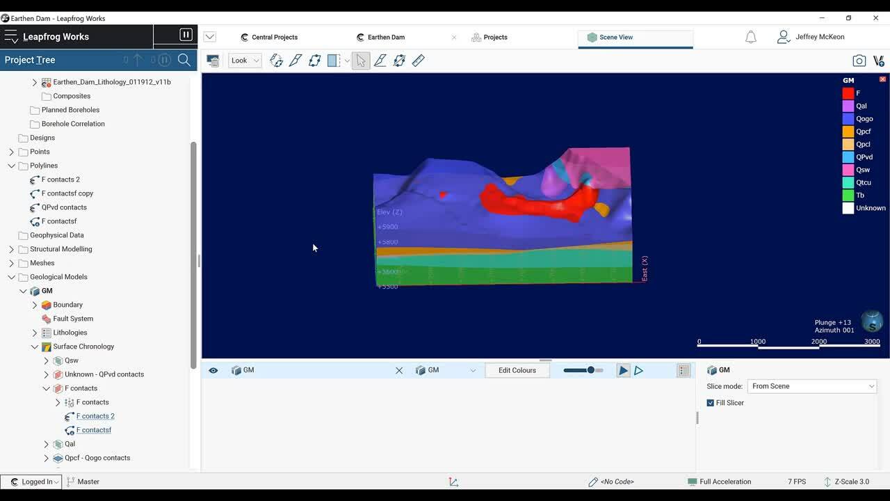
The interface is split up into three different components.

[00:06:20.230]
You have your project tree, where all of your data

[00:06:23.340]
is housed and organized.

[00:06:25.690]
You have your scene view which is where you visualize

[00:06:28.940]
your data and your object list or shape list

[00:06:32.860]
where whatever is visualized in the scene

[00:06:35.680]
appears just so you can keep track

[00:06:37.660]
of what you’re looking at.

[00:06:39.720]
Jumping over to the project tree.

[00:06:41.920]
To import data into any of these folders,

[00:06:45.910]
all you do is right click

[00:06:47.830]
where it gives you your import options.

[00:06:52.210]
For boreholes, this is showing up gray

[00:06:54.320]
because I already have them in the scene.

[00:06:58.120]
Just going to to pull this in really quickly.

[00:07:01.830]
So boreholes can be pulled in from an array

[00:07:03.550]
of different sources.

[00:07:05.150]
You can connect to local database like access, open ground,

[00:07:11.010]
a direct connection through open ground

[00:07:13.040]
or local files like CSV or text files.

[00:07:16.330]
You can also pull directly from Central,

[00:07:18.490]
which is sequence, cloud hosted system

[00:07:21.150]
for data and model management,

[00:07:23.670]
which is what I did in this case

[00:07:24.970]
that’s why there’s this little C icon right here.

[00:07:28.790]
So once the data is loaded into your project,

[00:07:32.200]
you can start to build these holistic representations

[00:07:36.080]
of your project area.

[00:07:38.520]
So Leapfrog works by introducing X, Y, Z data

[00:07:42.920]
and space where it then uses the radial basis function

[00:07:47.260]
or RBF, which is akin to dual creaking

[00:07:49.610]
to build implicit models.

[00:07:52.110]
So each point is weighted statistically

[00:07:54.550]
to create a best fit surface.

[00:07:57.290]
This can be a topographic surface,

[00:08:00.310]
a lithological contact surface, or a water table surface.

[00:08:06.300]
All objects you build are dynamically linked to the source

[00:08:09.610]
data indicated by these hyperlinks underneath the object.

[00:08:13.980]
So I built this topography in Leapfrog

[00:08:17.070]
using the Martis 10 ft point data.

[00:08:20.360]
If you click on the hyperlink, it will direct you

[00:08:23.390]
and the project tree to that source data.

[00:08:26.400]
So if I drag this and we can see that this surface

[00:08:30.600]
was created by interpolating between these points.

[00:08:35.690]
Another thing to mention

[00:08:37.800]
is that these are dynamically linked.

[00:08:40.570]
So if I were to change the source data, this object

[00:08:44.840]
that the source data was built from will reprocess,

[00:08:48.210]
and then in turn anything using the topography

[00:08:51.000]
and your downstream modeling processes

[00:08:53.660]
will also be reinterpreted.

[00:08:56.700]
So with this source data,

[00:08:58.040]
you can create your geologic models,

[00:09:00.500]
your water table models, numeric models, contaminant models,

[00:09:04.960]
all in these folders down here.

[00:09:07.920]
Really quickly, I’m just going to show

[00:09:10.840]
the geological model building process

[00:09:13.100]
for those who have not used Leapfrog Works.

[00:09:16.000]
So to build a model, and this works in any

[00:09:18.380]
of these modeling folders.

[00:09:21.470]
You right click, and I’m going to select

[00:09:23.633]
a new geological model, I’m also really quickly going

[00:09:27.490]
to pull my borehole data into the scene.

[00:09:36.134]
Okay, so here, I’m going to select my lithology,

[00:09:40.980]
my surface resolution, as well as the model extents,

[00:09:44.760]
you can set them manually, modify them in the scene

[00:09:47.970]
or select an object to enclose.

[00:09:50.930]
I’m just going to enclose my lithological data and click okay,

[00:09:57.330]
and then this will create your geological model.

[00:10:01.320]
So it’s comprised of your boundary,

[00:10:04.670]
which is what we just set, fault system,

[00:10:06.930]
if you have faults in your project, your lithology,

[00:10:11.140]
and probably the two most important folders,

[00:10:13.990]
surface chronology and your output volumes.

[00:10:17.770]
So initially it will create this unknown output volume

[00:10:21.410]
based on the model extents that we set with the upper bound

[00:10:25.890]
being the topographic surface.

[00:10:30.100]
To curve up this, let me make it a little more transparent.

[00:10:37.560]
To curve this up, we’re going to come

[00:10:39.700]
into the surface chronology folder and create some surfaces.

[00:10:44.980]
I’m just going to create one to show this process.

[00:10:48.780]
So there’s a bunch of different surfaces,

[00:10:50.730]
I’m going to select a deposit from base lithology.

[00:10:56.700]
Here I’m going to one second, I’m going to create a surface

[00:11:01.740]
for my, this purply blue unit.

[00:11:06.290]
This is just a sedimentary unit.

[00:11:08.880]
So I’m going to select that and select use contacts below.

[00:11:13.440]
This will then create a point for every lower boundary

[00:11:16.630]
contact of this Q-O-G-O unit and when I’m happy,

[00:11:22.520]
I’m going to click okay,

[00:11:25.050]
and that will generate our surface right here.

[00:11:29.420]
Drag that into this scene and we can see

[00:11:31.490]
that the surface honors our borehole data very well.

[00:11:35.610]
So I already have this model built,

[00:11:38.390]
so I’m just going to go ahead and clear the scene

[00:11:41.290]
and show you all of the surfaces that I created

[00:11:45.840]
using this lithological data.

[00:11:51.890]
So these surfaces, a majority of these surfaces

[00:11:54.580]
were created just using the contact information.

[00:11:59.100]
You can also incorporate other sources of information,

[00:12:01.560]
such as GIS lines or contacts at your surface.

[00:12:05.720]
You can introduce your own points in polylines

[00:12:11.600]
so in areas where data is sparse, such as over in this area,

[00:12:18.470]
some surfaces may blow out where you don’t want them to.

[00:12:23.920]
So for instance, this red surface

[00:12:26.860]
is my fill surface right here.

[00:12:31.283]
(keyboard clicking)

[00:12:39.164]
So originally the surface was blowing out all over this area

[00:12:43.470]
because there aren’t any holes.

[00:12:44.910]
So I just went in and manually constrained them

[00:12:48.830]
with these two polyline objects.

[00:12:56.401]
So we can see one polyline here, one right here, here,

[00:13:02.130]
and up here, just to make sure

[00:13:04.940]
that we are building something that is representative

[00:13:08.670]
of our project area.

[00:13:11.520]
So all that being said, I’m just going to clear this scene

[00:13:14.230]
and drag the geological model back into the scene.

[00:13:19.400]
So once those surfaces curve up, that unknown output volume,

[00:13:23.410]
will then generate these different volumes for your units.

[00:13:29.810]
So once the model is built, it can then be published

[00:13:32.210]
to Central for peer review.

[00:13:34.700]
Central is one of our solutions,

[00:13:37.050]
it’s a system for data and model management.

[00:13:40.060]
It’s a store environment that can consistently version track

[00:13:43.040]
data coming into the project from the field

[00:13:45.350]
and dynamically link it.

[00:13:47.700]
To publish, you just click on this little Central icon

[00:13:50.650]
in the bottom left and select publish.

[00:13:55.080]
Here you have the option of selecting what you would like

[00:13:57.290]
to publish as well as the ability to include

[00:14:01.740]
the entire project so people can copy it down

[00:14:04.420]
on their server and work on it.

[00:14:06.760]
You can also select which stage this publication is.

[00:14:13.230]
I already have one published, so I’m just going

[00:14:14.930]
to directly jump into the Central server to do so.

[00:14:18.630]
You come over to Central projects and select open portal,

[00:14:22.320]
and then you’re going to select your project.

[00:14:25.680]
So I’m going to be jumping in and out

[00:14:27.240]
of Central in this webinar.

[00:14:28.890]
So I’m going to come back to all of the version tracking

[00:14:32.010]
and other functionality, but right now,

[00:14:34.200]
I want to highlight the Central data room.

[00:14:37.740]
That is just this little files tab here.

[00:14:41.380]
So the Central data room is a cloud hosted system

[00:14:45.070]
that allows you to organize your project data

[00:14:47.100]
and dynamically link it to specific objects in your project.

[00:14:53.210]
Here, you can add data as it comes into the field,

[00:14:55.500]
as well as version track it.

[00:14:59.757]
In this instance, I have an additional

[00:15:00.990]
roundup borehole information.

[00:15:03.080]
So I’m going to jump into my borehole data,

[00:15:07.260]
I’m just going to select my collar.

[00:15:09.280]
If you want to update an object,

[00:15:11.710]
you click on it and then come over

[00:15:13.490]
and select upload new version.

[00:15:17.060]
So I’m just going to click on the new collar information

[00:15:20.650]
and click Okay, and then that will allow you

[00:15:24.870]
to version track right here.

[00:15:27.530]
So I already did that for these two,

[00:15:29.630]
so I’m just going to jump back into Leapfrog.

[00:15:36.160]
When the data in Central has been updated,

[00:15:38.660]
a little clock icon will appear

[00:15:40.680]
in the project tree next to the object.

[00:15:45.090]
This indicates that this is out of date

[00:15:47.330]
and will need to be reloaded.

[00:15:50.430]
To do so, I’m just going to pull this in

[00:15:52.250]
so we can visualize this and maybe turn this transparency.

[00:16:02.290]
Okay, so as we can see, the little clock icon is here.

[00:16:06.370]
So I’m just going to right click on this object

[00:16:09.850]
and here you have the option to reload

[00:16:12.290]
from the latest file version, or you can reload

[00:16:15.270]
from any of the files in your file history.

[00:16:18.870]
In this case, I’m just going to reload

[00:16:20.830]
the latest file version, and that will prompt this screen.

[00:16:28.710]
So here we can see our mappings of our collar information.

[00:16:34.420]
It’s going to retain the mappings

[00:16:37.070]
that you had in the last import,

[00:16:39.670]
so I’m happy with this, I’m just going to click finish.

[00:16:42.540]
And now that is going in and reprocessing everything

[00:16:45.870]
that was dynamically linked to this portal information.

[00:16:50.180]
So here we can see that new round of boreholes is in,

[00:16:55.340]
and it is now reprocessing our geological model.

[00:17:02.130]
So throughout the life cycle of the project,

[00:17:04.950]
we will constantly be bringing in more and more information.

[00:17:09.150]
Like we just brought in a new round of drilling

[00:17:11.870]
and the project will consistently,

[00:17:14.110]
dynamically update throughout this entire process.

[00:17:18.320]
This can be geophysical data from Oasis montaj,

[00:17:22.080]
which is our geophysical suite of tools,

[00:17:24.970]
geo-technical analysis through GeoStudio

[00:17:27.500]
or geotechnical suite of tools

[00:17:29.610]
or any other suite of software

[00:17:31.380]
that you’re pulling information from.

[00:17:34.820]
And that information will go into its appropriate folders.

[00:17:39.980]
We can also, we have many APIs

[00:17:42.300]
with different software companies.

[00:17:44.070]
So flow models, we can create MODFLOW and FEFLOW grids

[00:17:49.170]
in Leapfrog to be used

[00:17:51.210]
in these respective software packages.

[00:17:53.750]
So I updated the model again,

[00:17:55.990]
and I’m going to go ahead and publish.

[00:17:59.900]
So I’m just going to jump back into the portal.

[00:18:04.170]
So again, here we can see the latest model

[00:18:07.360]
that publishing event that I just did.

[00:18:10.740]
We can see what changes have occurred,

[00:18:13.000]
who’s made these changes and established a peer review

[00:18:15.860]
process, as well as version track.

[00:18:20.400]
In the browser, you can also limit

[00:18:22.810]
who has access to these models

[00:18:25.610]
and you can connect stakeholders,

[00:18:28.060]
other people working on the model,

[00:18:29.460]
other modelers, geophysicists, geologists,

[00:18:32.380]
so that everybody can collaborate on building

[00:18:35.240]
the best representation or a digital twin

[00:18:37.430]
of your project area.

[00:18:38.680]
So in this browser as well,

[00:18:41.180]
it’s not only the raw data files and the data room

[00:18:44.910]
that we looked into previously, or the version tracking,

[00:18:48.660]
but you can also allow intellectual exchanges

[00:18:52.350]
between modelers and stakeholders

[00:18:54.690]
to actively peer review in real time.

[00:18:57.630]
So anybody connected to this project will get notifications

[00:19:01.330]
when any updates occur and those notifications appear

[00:19:06.532]
in this bell icon.

[00:19:08.680]
So if I click here, I can see that a day ago,

[00:19:12.160]
Steven Donovan commented on the master branch.

[00:19:16.550]
So if I click on that notification,

[00:19:18.000]
it will bring up the model that this applies to.

[00:19:22.230]
So we can see here, this is one of the older revisions.

[00:19:26.810]
So we can see here that he said,

[00:19:29.410]
film material looks to be blowing out,

[00:19:31.160]
please constrain the model.

[00:19:34.160]
And so that’s what I did.

[00:19:35.420]
I went in and I fixed this area.

[00:19:37.590]
I republished and said that I’ve fixed the blow out here.

[00:19:41.750]
So when I replied to his comment,

[00:19:43.170]
he will also get those notifications.

[00:19:45.550]
So this is the Central web browser.

[00:19:47.590]
Really quickly, I’m going to jump over

[00:19:49.570]
to our Central desktop application.

[00:19:53.030]
It has pretty similar functionality,

[00:19:55.060]
it’s just a little more built out.

[00:19:57.430]
So here is the Central browser.

[00:19:59.320]
Again, it is a desktop application.

[00:20:01.620]
Here you can see all of your project revisions.

[00:20:03.900]
It’s very similar to the web browser, but again,

[00:20:06.840]
it has a bit more functionality.

[00:20:08.420]
I’m going to go ahead and click on the most recent version.

[00:20:11.610]
And here you have the ability to pull any

[00:20:14.670]
of these objects into the scene.

[00:20:23.790]
The feature that I wanted to highlight

[00:20:25.090]
is the ability to actively compare different models,

[00:20:28.040]
different objects that can be applied to boreholes,

[00:20:31.220]
faults, lithological units,

[00:20:33.750]
and allows you to compare your interpretations

[00:20:35.900]
and see how they’ve changed over time.

[00:20:37.940]
So for this exercise, I’m going to focus on my fail unit.

[00:20:44.130]
To go ahead and compare this to a previous revision,

[00:20:46.320]
you just come to the top and select

[00:20:47.870]
this compare revisions button.

[00:20:51.420]
You’re going to come over and select the revision

[00:20:53.560]
that you want to compare this to.

[00:20:55.860]
I’m going to select my first revision

[00:20:59.100]
and then going to modify the appearance of the object.

[00:21:04.310]
I’m just going to turn wireframing on for the older revision.

[00:21:08.080]
That way we can see those differences.

[00:21:11.930]
So here we can see that the wireframe fill object

[00:21:17.100]
is the older revision and we can see

[00:21:19.220]
that this is that big blowout area that my colleague

[00:21:22.790]
previously commented on to fix, which is what we did.

[00:21:27.628]
And we can also see here that the additional round

[00:21:29.320]
of drilling also modified this object.

[00:21:31.540]
So once we’ve decided that this fail unit

[00:21:35.050]
and our entire model is at the highest geological certainty,

[00:21:38.970]
we can go ahead and jump back over.

[00:21:42.670]
And now that this model is validated,

[00:21:45.580]
you can change the stage to approved,

[00:21:48.690]
which will update the project and then notify everybody

[00:21:51.100]
attached to the project that this model is now approved.

[00:21:54.610]
So now I’m going to switch back over to Leapfrog.

[00:21:57.940]
Now that my project is approved

[00:22:00.250]
and the geological model has been validated,

[00:22:03.150]
I can move forward with my geo-technical analysis,

[00:22:07.760]
just going to jump into this scene view.

[00:22:11.150]
I want to do a slope stability and SEEP analysis

[00:22:13.580]
along my dam axis, so I’m going to need to create

[00:22:16.180]
a few cross sections along this chainage.

[00:22:19.360]
This yellow line right here is loaded into my GIS.

[00:22:24.660]
This is some vector data that has been draped

[00:22:27.560]
onto my typography along with the map.

[00:22:31.210]
To go ahead and build cross sections along this,

[00:22:33.170]
I’m going to come down to the cross sections

[00:22:35.090]
and contours folder, right click,

[00:22:37.410]
and then this is going to give me multiple options

[00:22:40.500]
for my cross sections.

[00:22:42.570]
Because I want to make cross-sections along this chainage,

[00:22:44.720]
I’m going to select new alignment serial section,

[00:22:50.180]
and here it’s going to give me the ability

[00:22:53.570]
to select a new polyline or an existing one.

[00:22:56.850]
I’m just going to go ahead and select the existing one.

[00:23:00.060]
And here we can see that these cross sections

[00:23:02.240]
are being populated along this chainage.

[00:23:07.350]
I’m going to modify some of these parameters,

[00:23:10.670]
going to change the width and the height to 500.

[00:23:16.360]
I’m going to move the line or move the cross sections

[00:23:20.170]
down a bit and then I’m going to change my chainage,

[00:23:25.350]
spacing to something like 250.

[00:23:30.900]
And when I am happy with this,

[00:23:32.980]
I’m just going to zoom in to increase this transparency a bit.

[00:23:41.040]
It looks like there a little bit below,

[00:23:42.830]
so I’m just going to modify this and that looks good.

[00:23:50.360]
And we can see here that they all say F,

[00:23:52.470]
meaning that this is the front of the cross section,

[00:23:55.660]
or the back of the cross section says B for back.

[00:23:59.550]
So when I’m happy with this,

[00:24:00.560]
I’m going to go ahead and click okay.

[00:24:03.610]
And that’s going to create the sections right here.

[00:24:08.730]
First, I’m going to need to evaluate

[00:24:10.940]
my geological model onto my sections.

[00:24:14.090]
So I’m going to right click on these and select evaluations.

[00:24:20.400]
And I’m just going to pull over my geological model

[00:24:23.720]
and click okay, and then that will evaluate

[00:24:29.310]
the geological model onto all of these sections.

[00:24:34.040]
Now that is done, I’m going to pull these into the scene

[00:24:40.110]
and I’m going to turn these off

[00:24:44.060]
and here we can see the geological model

[00:24:46.830]
now evaluated onto all of these sections.

[00:24:52.070]
I am then going to create a section layout.

[00:24:57.340]
So to do this, I just right click on the cross sections

[00:25:01.000]
and select new masters section layout.

[00:25:03.890]
And here we have a bunch of different options

[00:25:07.090]
for our cross sections.

[00:25:08.320]
I’m going to select my model

[00:25:14.230]
and I’ll just keep the default settings

[00:25:16.510]
as they are and click okay.

[00:25:18.490]
And so now this is populated.

[00:25:21.180]
I’m just going to move some things around.

[00:25:23.750]
To move things in the section around,

[00:25:25.430]
you just drag and drop, maybe move my sections down a bit,

[00:25:34.890]
drag this to the center.

[00:25:38.440]
I’m also going to want to evaluate

[00:25:41.740]
my boreholes onto my section.

[00:25:44.260]
So to do that, you just come to boreholes in this list,

[00:25:49.450]
right click and select add boreholes.

[00:25:53.765]
I’m going to select my lithology data.

[00:25:57.340]
And here we can select all of the boreholes or filter

[00:26:00.300]
by a minimum distance.

[00:26:03.210]
In this case, I’m going to filter by maybe 125

[00:26:15.870]
and then check this on and click okay.

[00:26:20.620]
So now my boreholes are on.

[00:26:24.830]
And when you are happy with your section layout,

[00:26:29.580]
you just click save and then right click

[00:26:33.590]
on your master section layout copy too,

[00:26:37.270]
and just go ahead and select all of the cross sections

[00:26:42.750]
you just created.

[00:26:43.760]
And once that is done processing,

[00:26:45.530]
you can drag this into the scene.

[00:26:48.110]
And here are multiple cross sections

[00:26:52.010]
with your section layout applied along this chainage.

[00:26:58.440]
So now that my cross sections are created,

[00:27:00.820]
I’m just going to grab a few,

[00:27:01.970]
put them in the data room for Kathryn to pull down

[00:27:04.790]
and do the slope stability analysis, and the SEEP analysis.

[00:27:09.550]
You can export these cross sections in an array

[00:27:11.670]
of different exchange formats.

[00:27:13.360]
You just right click and select export,

[00:27:16.630]
select your geological model

[00:27:18.100]
and here are the exchange formats that we offer.

[00:27:21.630]
We can do DXF, DWG as well as DGN.

[00:27:26.770]
So I’ve already exported these

[00:27:28.330]
and thrown them in the data room.

[00:27:30.050]
So at this point, I’m just going to hand it over

[00:27:32.610]
to Kathryn to run that analysis.

[00:27:37.760]
<v Kathryn>Thanks, Jeff.</v>

[00:27:39.430]
As Jeff demonstrated, he published cross sections

[00:27:41.950]
from his geological model of the tailings embankment

[00:27:44.570]
to Central and granted me access to this project.

[00:27:47.900]
Subsequently, I have opened up Central through my internet

[00:27:50.590]
browser and can now click on this project

[00:27:53.100]
to view its history.

[00:27:56.710]
I see there are two branches of the project.

[00:27:59.130]
I wish to use the cross sections from the master branch

[00:28:01.670]
that were approved and uploaded by Jeff.

[00:28:06.110]
These cross sections were placed in the files associated

[00:28:08.560]
with the project under geotechnical cross sections.

[00:28:12.340]
Here, I will select each one and download them

[00:28:15.380]
so I can use them to create my project geometry.

[00:28:28.800]
In Central, I can also view the positioning

[00:28:30.840]
of these cross sections in the overall geological model,

[00:28:34.130]
by going back to the overview tab

[00:28:36.870]
and selecting the master project file,

[00:28:39.190]
which opens it in the project scene.

[00:28:43.360]
Here, I will toggle on the output volumes

[00:28:45.360]
from the geological model,

[00:29:14.200]
and then select the three cross sections

[00:29:18.330]
at 2500, 2750 and 3000.

[00:29:32.350]
I see that the cross sections cut through the curved section

[00:29:34.990]
of the tailings embankment.

[00:29:45.890]
In GeoStudio, I have created a new project

[00:29:48.240]
with metric units.

[00:29:50.120]
In this file, I will add three, two-dimensional geometries,

[00:29:54.320]
one for each of the cross sections

[00:29:55.970]
that I have just downloaded from Central.

[00:30:04.405]
I will name them according to the position

[00:30:05.710]
of the cross section in the geological model

[00:30:22.210]
and close the defined project dialogue.

[00:30:25.750]
In the first two-dimensional geometry,

[00:30:27.710]
I will select file import, go to my downloads folder

[00:30:31.760]
and select the cross section at 2500.

[00:30:35.860]
I will ensure that the materials are imported

[00:30:37.930]
from the layer names and turn off the option

[00:30:40.510]
to translate the cross section horizontally

[00:30:42.740]
to start at X is equal to zero.

[00:30:46.210]
You will notice that the analysis details are very small,

[00:30:49.760]
and so I will go to define scale

[00:30:52.190]
and change the reference scale ratio to one to 3000.

[00:31:00.610]
Following the same procedure,

[00:31:02.070]
I will import the cross sections at 2750 and 3000

[00:31:06.920]
to the corresponding GeoStudio geometries.

[00:31:33.540]
My geometry definition is now complete.

[00:31:36.470]
The next step for setting up a GeoStudio analysis

[00:31:39.360]
is to define the physics.

[00:31:41.520]
In order to do so, I must first establish

[00:31:43.990]
what types of analysis I wish to simulate

[00:31:46.270]
on the model domain.

[00:31:48.020]
This is done in the defined project window.

[00:31:52.110]
I wish to simulate transient,

[00:31:53.550]
poor water pressure conditions.

[00:31:55.590]
To do so, I will first add a steady state SEEP/W analysis,

[00:31:59.460]
which establishes my initial conditions

[00:32:01.450]
throughout the domain.

[00:32:03.570]
Then I will add a transient CPW analysis as its child.

[00:32:08.610]
I will set the duration of the transient analysis to 60 days

[00:32:12.410]
with half day time steps that are saved every four steps.

[00:32:17.650]
I will add similar analysis

[00:32:19.190]
to the other two geometries in the project file.

[00:32:57.930]
Once I’ve finished adding the analysis,

[00:32:59.860]
I must now specify the material properties

[00:33:02.350]
to complete the definition of the physics on the domain.

[00:33:06.300]
I’ve already copied the material properties

[00:33:08.030]
over from a previous GeoStudio file

[00:33:09.950]
conducted on the same project site.

[00:33:13.450]
Note that some of the materials use the saturated only

[00:33:15.880]
material model while others closer to the ground surface

[00:33:18.870]
use the saturated-unsaturated material model.

[00:33:24.070]
The next step in setting up our GeoStudio project

[00:33:26.350]
is to define the boundary conditions

[00:33:28.110]
for the SEEP/W analysis.

[00:33:30.860]
There are two default hydraulic boundary conditions.

[00:33:34.320]
The drainage boundary represents the conditions

[00:33:36.620]
along a potential seepage face.

[00:33:39.740]
I will use this on the downstream side of the embankment.

[00:33:44.350]
I must also add a new boundary condition that represents

[00:33:46.880]
the water level in the tailing storage facility.

[00:33:50.840]
I will add a new water total head boundary condition

[00:33:54.140]
to find by a function that represents

[00:33:56.700]
the changing water level over time.

[00:34:05.900]
To define the function, I will copy the field data

[00:34:08.530]
for the water surface elevation over time

[00:34:11.640]
into the function definition window.

[00:34:32.768]
I can now apply the boundary conditions to the model domain.

[00:34:36.550]
I will select the apply to multiple analysis option

[00:34:38.950]
in the draw Boundary Conditions dialogue,

[00:34:41.250]
and apply my boundary conditions to both the steady state

[00:34:44.300]
and transient seepage analysis.

[00:35:19.300]
The last step of defining the seepage analysis

[00:35:21.680]
is to set the finite element mesh size,

[00:35:24.420]
which I will specify as five meters.

[00:35:34.300]
I’m now ready to solve the analysis.

[00:35:56.780]
When solved, the file automatically changes to results view.

[00:36:00.480]
I will add an ISO surface at a pore water pressure value

[00:36:03.370]
of zero kPa to represent the position

[00:36:05.830]
of the free attic surface throughout the domain.

[00:36:09.400]
I could also turn on the total head

[00:36:11.020]
or pore water pressure contours.

[00:36:20.410]
In the transient analysis, I can view the results over time

[00:36:23.540]
by clicking through the timestamps shown

[00:36:25.380]
in the result times window.

[00:36:43.990]
I can now add a SLOPE/W analysis to determine the stability

[00:36:46.810]
of the system as the water level changes.

[00:36:59.350]
This project includes both soil and rock materials,

[00:37:01.400]
which can be represented with a wide range

[00:37:03.360]
of material models available in SLOPE/W.

[00:37:08.010]
I have already done so in a different GeoStudio file.

[00:37:13.280]
You will note that as the water level in the tailings

[00:37:16.220]
facility rises, the critical factor of safety decreases.

[00:37:29.520]
Once I’ve completed my model in GeoStudio,

[00:37:31.970]
I can export my analysis cross section to a DXF or DWG file

[00:37:37.000]
that could be imported back

[00:37:38.390]
into the original Leapfrog Works project file.

[00:37:46.410]
I will reopen Central and update the cross sections

[00:37:49.210]
in the project data files.

[00:38:18.977]
I can also upload the GeoStudio project file,

[00:38:21.240]
so my colleagues have access to it.

[00:38:45.910]
We’ve now reached the end of this webinar.

[00:38:48.130]
Please take the time to complete the short survey

[00:38:50.190]
that appears on your screen, so we know what types

[00:38:52.260]
of webinars you’re interested in attending in the future.

[00:38:55.890]
Thank you very much for joining us

[00:38:57.430]
and have a great rest of your day.

[00:38:59.430]
Goodbye.