Industry Best Practices for Processing Onshore UXO Geophysical Data

New and experienced users alike will walk away with practical tips to improve their use of UXO Land.

Presenter Information
Laura Quigley, Technical Analyst, Seequent

Laura received her Bachelor of Science degree in Geophysics from Memorial University in Newfoundland and Masters of Science in Geophysics from the University of Toronto. Her professional career started with Fugro Airborne Surveys, processing and interpreting airborne geophysics data. She then worked for a marine seismic company where she participated in a number of research cruises to Greenland.

After completing her Masters degree in 2013, Laura moved to Australia where she worked for the University of Queensland on seismic projects for unconventional coal seam gas development, then moved to the Queensland University of Technology where she spent several years researching geodynamical processes through analogue modelling. Laura returned to Toronto, Canada in January 2020 to join Seequent as a Technical Analyst.

Overview

Video Transcript

[00:00:00.420]<v Laura Quigley>Hi everybody, my name is Laura Quigley</v>

[00:00:02.930]and I’m a technical analyst at Seequent.

[00:00:05.660]On behalf of Seequent I would like to welcome you

[00:00:07.570]to today’s webinar on industry best practices

[00:00:09.910]for processing on-shore UXO geophysical data.

[00:00:13.770]So today I’ll be teaching you some time-saving tips

[00:00:16.060]to make your workflows in oasis montaj more efficient

[00:00:20.370]and I will focus on UXO land.

[00:00:22.410]So firstly I will go over the UXO land workflow overview.

[00:00:27.340]Next I will look at four modeling target anomalies.

[00:00:30.770]Applying heading corrections, using instrument tests,

[00:00:35.110]footprint coverage and our footprint coverage tool.

[00:00:38.810]Next we will look at targets and how to pick

[00:00:41.240]positive peak targets from a profile and data linking.

[00:00:46.240]We’ll learn to manage our targets

[00:00:48.170]by adding emerging targets.

[00:00:51.170]Then we look at picking peaks from a grid,

[00:00:54.070]so I’ll look at the Blakely method.

[00:00:56.740]And then finally I look at magnetic dipoles

[00:00:59.050]for picking targets through a grid and using your profile.

[00:01:05.980]Okay, so the UXO land workflow overview.

[00:01:10.680]Okay so first of all I’m going to look at

[00:01:11.970]a general UXO land workflow,

[00:01:14.830]so we begin by importing our data into oasis montaj.

[00:01:18.620]So under data preparations

[00:01:19.890]I have planned survey in instrument tests.

[00:01:22.690]So instrument tests are run using your survey instrument

[00:01:26.590]and can be processed in oasis montaj.

[00:01:29.520]And planning a survey can be done prior to

[00:01:32.040]completing your survey

[00:01:33.550]and this is just a feature we have that allows you

[00:01:35.430]to plan your survey.

[00:01:38.580]Okay, so once you have your data imported

[00:01:40.570]and your instrument test processed,

[00:01:42.710]you can begin by looking at your survey data

[00:01:44.970]and doing some data reduction.

[00:01:46.420]So despiking, smoothing your data

[00:01:48.520]and cleaning up the channels.

[00:01:50.950]Next we can apply data corrections,

[00:01:52.560]so base station corrections, heading corrections

[00:01:55.630]and for gradiometry surveys,

[00:01:57.200]we can do a sensor offset correction.

[00:02:00.030]And also at this stage, when we do the sensor offset

[00:02:02.290]we have the option to combined our sensors into

[00:02:05.080]one survey or into one channel.

[00:02:07.830]So this will enable us to grid our magnetic data

[00:02:10.790]’cause it’s in one channel.

[00:02:17.120]Okay, so now we want to pick targets,

[00:02:19.180]so for magnetic data, you would generally calculate

[00:02:21.898]analytical signal.

[00:02:23.720]and from that we could use the Blakely method to pick peaks.

[00:02:27.150]We can also use electromagnetic data and the Blakely method

[00:02:30.450]to pick electromagnetic peaks.

[00:02:34.040]And we can also pick targets using dipole,

[00:02:36.540]so total magnetic field data,

[00:02:38.140]we can look at picking targets from grids and from profiles.

[00:02:42.990]So once you have your targets picked,

[00:02:44.820]we’re able to manage the target list.

[00:02:48.050]So this could be emerging targets,

[00:02:49.640]so if there’s a cluster of targets you see

[00:02:51.310]that you’d like to merge into one, you can do that.

[00:02:54.130]You can add or remove individual targets

[00:02:56.890]and you can also bring in additional data

[00:02:58.420]to cross-reference your targets.

[00:03:02.070]Next, we have the option to do some depth modeling,

[00:03:04.590]so this involves calculating a target size.

[00:03:06.840]So this is a window around your anomaly

[00:03:09.450]and this window will be used for your oiler deconvolution

[00:03:12.110]in which you will calculate size and apparent depth.

[00:03:16.040]Batch fit you can also calculate your parent depth

[00:03:18.530]and size and a magnetic moment

[00:03:23.210]and then finally we can export our target lists.

[00:03:29.370]So for beginners or just as a refresher,

[00:03:31.690]you can go on my seequent.com/learning.

[00:03:35.690]So within this webpage we have a list of learning paths

[00:03:40.020]for all our oasis montaj extensions

[00:03:42.900]and here I’ve highlighted the UXO land.

[00:03:45.530]So if you go in here,

[00:03:46.770]you’ll see a learning path for this tool.

[00:03:54.410]Okay, so first I’m going to look at

[00:03:55.540]forward modeling target anomalies.

[00:04:01.420]Okay, so now I’m in oasis montaj

[00:04:03.294]and I have a UXO land project open

[00:04:07.190]with a bunch of data already loaded,

[00:04:09.260]so this is what I’ll be using as an example today.

[00:04:12.690]And the UXO land menus are loaded on top here,

[00:04:15.580]so we have data preparation, parameter determination,

[00:04:18.330]target inversion and target management

[00:04:20.970]and I’m going to speak a bit about each of these today.

[00:04:24.140]So the first thing I wanted to show you

[00:04:25.910]was forward modeling.

[00:04:27.610]So forward modeling is a great way

[00:04:29.100]to efficiently calculate a range of EM

[00:04:31.910]or magnetic signatures for a range of targets

[00:04:35.260]and sampling scenarios.

[00:04:37.640]So you don’t really need to have any data

[00:04:39.500]to do any forward modeling in oasis montaj.

[00:04:43.370]So I will show you how to use this tool,

[00:04:46.270]so it’s under target inversion, calculate forward models.

[00:04:51.490]So we can choose from a sensor type,

[00:04:53.240]we can use magnetics or EM,

[00:04:55.470]so we have the EM61 sensor here.

[00:05:00.440]You can choose to output your data to a database.

[00:05:04.190]And then here you can define your targets.

[00:05:07.610]You can also add some background noise,

[00:05:09.410]so if you have a database

[00:05:10.510]that’s relatively quiet in your area,

[00:05:12.690]that’ll just add that bit of noise to your model,

[00:05:15.230]you can do that.

[00:05:16.910]And we can calculate an IGRF,

[00:05:18.840]so a background magnetic field in our survey area

[00:05:22.047]and I’ll show you how to do that.

[00:05:25.280]Okay, so I’ll, first of all show you

[00:05:28.190]how to calculate the IGRF,

[00:05:29.500]so then then this tab here will be populated automatically.

[00:05:32.780]So I’m going to close this tool

[00:05:34.840]and also under target inversions tools, IGRF calculations.

[00:05:42.420]Okay so the database I’m going to be working with

[00:05:44.820]is APG mag blind.

[00:05:47.840]So our survey area this is the name here APG,

[00:05:51.040]so Aberdeen Proving Ground.

[00:05:53.030]The sensor type is mag

[00:05:54.600]and the survey block is called blind, okay.

[00:05:59.810]And then you specify the lots in long channels.

[00:06:02.420]So from a dropdown list,

[00:06:03.970]you just search for those in your database.

[00:06:06.420]And if you don’t have those in your database,

[00:06:08.200]for example if you just have UTM coordinates,

[00:06:10.560]I can show you how to create your lat and long channels,

[00:06:14.030]which I’ll do quickly after the forward modeling.

[00:06:17.730]Okay, so then you just click IGRF

[00:06:20.510]and you should have values calculated.

[00:06:23.010]So you have the field strength, so it’s roughly 45,000

[00:06:25.920]and you have your magnetic inclination and declaration here

[00:06:29.780]and then I just simply click close.

[00:06:33.250]So now under my forward modeling,

[00:06:37.410]this tab here should be populated and it is.

[00:06:42.200]Okay, so I’ll go through the target definition,

[00:06:44.460]we can set up a one, two or three targets

[00:06:46.710]to have in our model.

[00:06:48.640]I’m going to set the origin of the first target

[00:06:50.840]at zero, zero and the size.

[00:06:53.960]So we have a list of munitions here

[00:06:55.730]that you can use to forward model.

[00:06:58.330]So I’ll use an 81 millimeter for example.

[00:07:02.520]Okay and the distance is the distance below the sensor,

[00:07:06.130]so your target distance below the ground,

[00:07:09.450]plus your sensor height.

[00:07:11.050]So say if I’m carrying a sensor at two meters

[00:07:14.850]and my targets at two meters below the surface,

[00:07:17.640]I can just put four here.

[00:07:20.240]And the inclination I’ll do a vertical targets,

[00:07:22.690]so I will use 90 and I’ll choose a declaration of zero.

[00:07:28.330]Okay and this is really all we need

[00:07:30.320]to run our forward model.

[00:07:33.140]We can add noise, we can add additional targets

[00:07:36.440]and we can also loop through various parameters,

[00:07:38.840]so if I wanted to increase the distance for example.

[00:07:42.970]First of all I’ll show you this, so I just click run

[00:07:48.790]and you get a grid and a profile.

[00:07:52.940]So I’m going to change the color bar of my grid,

[00:07:56.540]I want to be able to see a bit more.

[00:07:59.160]So under color bar,

[00:08:01.900]I can select a min and max.

[00:08:03.580]So I have mine set at a manual scale,

[00:08:05.480]so that’s why the colors didn’t really

[00:08:09.080]display the data best.

[00:08:12.270]So if I clicked automatic scale first of all.

[00:08:23.290]Okay, so I just ran that using an automatic scale

[00:08:25.760]and I see a bit more definition.

[00:08:28.090]I can also change this to manual and keep it set.

[00:08:32.190]For example, if I’m going to loop through some data

[00:08:34.520]and I want to see all the data at the same color bar,

[00:08:36.930]I can do that.

[00:08:38.260]I’ll set that now, ’cause we have a range of roughly

[00:08:41.471]what we’d like, so negative 0.1 is our minimum,

[00:08:47.730]I’m just looking at the profile and at the color scale here.

[00:08:53.070]Maximum we can put at one

[00:09:00.919]and then I’ll just click okay

[00:09:03.070]and I’ll run that just to see how it looks.

[00:09:11.670]Okay.

[00:09:14.970]Next I’m going to show you how to create a loop.

[00:09:18.000]So this way we can see how the target signature will change

[00:09:21.690]when our parameters changed.

[00:09:24.540]So I’m going to select my first targets

[00:09:28.610]and the parameter I’d like to loop through

[00:09:30.020]is distance below the sensor.

[00:09:32.400]You can also loop through target size

[00:09:34.720]or inclination or declination.

[00:09:39.660]So down here I’ve entered a target size,

[00:09:41.650]so this is my target window that I’d like to model.

[00:09:45.320]I’ve just chosen 10, you can increase or decrease this

[00:09:49.390]and it would affect the anomaly that you see on the screen.

[00:09:55.220]I’m going to set the minimum to four

[00:09:59.370]and I’m going to increment by half a meter

[00:10:02.000]and I’m going to go down to eight meters.

[00:10:05.450]And then if I click run loop,

[00:10:07.840]I should be able to see how the anomaly changes with depth.

[00:10:18.304]So you can see that the signature

[00:10:19.850]on the grid gets a lot weaker

[00:10:22.160]and the profile amplitude gets lower.

[00:10:33.720]So this is just a great way to see

[00:10:35.810]how your sensor height for example,

[00:10:37.490]affects the anomaly reading you’re going to get.

[00:10:40.810]So I’ve chosen a pretty deep target here,

[00:10:43.870]so we won’t get much of a signature from that.

[00:10:49.990]And also my color scale has been set to manual,

[00:10:53.980]so it’s going to remain at these values.

[00:10:56.690]I’m just going to bring that down a bit to say 0.7.

[00:11:03.566]Okay, so next, I’m going to add a second target

[00:11:08.270]say two meters away and let’s add a 20 millimeter.

[00:11:15.370]And we’ll start at four and I’ll bring this back to four

[00:11:19.560]where we started for the first one

[00:11:22.430]and I’ll use the same orientation

[00:11:26.660]and I’m going to increment target one

[00:11:31.210]through these loops as well and see the response.

[00:11:40.340]Okay, so I’m going to turn the looping off

[00:11:42.160]and just take a look at the response

[00:11:43.760]for a single timestamp for the both for two of the targets.

[00:11:49.280]Okay, so we see that a smaller target over here,

[00:11:51.710]you can actually barely pick it up.

[00:11:54.920]Let’s see if I added similar sized, the exact same target

[00:12:01.600]two meters away and we can see what that looks like.

[00:12:10.360]Okay, so there’s many options you can do here,

[00:12:12.340]you can change your size of your target,

[00:12:15.180]you can change your target depths,

[00:12:16.640]you can change the dipole moments of your target.

[00:12:25.510]And it provides valuable information,

[00:12:27.070]so for example if you’re going

[00:12:28.750]to look for 81 millimeters at a site,

[00:12:31.800]you’d like to know what height you have to hold your sensor

[00:12:38.520]in order to be able to detect these.

[00:12:41.010]And also if you had two targets close to each other,

[00:12:44.360]would that appear as a single anomaly on a map?

[00:12:47.090]So this type of information is really valuable

[00:12:49.320]and it’s a really good tool to prepare for our survey.

[00:13:05.342]I can save changes.

[00:13:08.040]And like I said you can refer back to these maps,

[00:13:10.050]so you have a profile map and the map manager here

[00:13:14.720]allows you to turn off or turn on

[00:13:16.140]various aspects of your profile.

[00:13:21.570]And then you also have

[00:13:26.310]a grid of your data, your anomaly that you just modeled.

[00:13:35.310]Okay, so if you have a database

[00:13:38.780]that you’d like to calculate, use to calculate the IGRF

[00:13:42.810]and it doesn’t have a lat and long channel, such as here.

[00:13:47.970]I’ll just show you how I created those,

[00:13:49.160]so when I initially had this database,

[00:13:50.700]it had the UTM coordinates which is great,

[00:13:53.290]but I’m just going to show you how to convert to lat, long

[00:13:55.670]which is needed to calculate the IGRF.

[00:13:58.990]So under coordinates,

[00:14:01.410]you can say new projected coordinate system.

[00:14:05.740]Okay, so you give it your current coordinate system,

[00:14:07.890]which would be your UTMs.

[00:14:12.540]And then again you specify the current coordinate system,

[00:14:15.250]so it’s projected x, y in to a UTM zone 23

[00:14:19.820]and the data (indistinct) then you click, okay.

[00:14:24.220]Here’s where you create your channel, so you give it a name.

[00:14:26.750]I called it long and lat.

[00:14:31.910]And then for this window you select geographic lat long,

[00:14:35.420]so this will project your UTMs back to lat longs.

[00:14:39.740]And then if you click okay,

[00:14:43.810]you will get these two channels in your database.

[00:14:46.700]And this is degrees, minutes, seconds, decimal degrees

[00:14:50.120]or decimal seconds.

[00:14:51.920]You can change the format,

[00:14:54.150]so I can go from geographic format to normal

[00:15:00.460]and that’s just decimal degrees,

[00:15:02.550]this is just various ways to display your lat longs.

[00:15:10.470]Now I’m going to look at applying heading correction

[00:15:12.540]using your instrument tests.

[00:15:17.450]Okay, so next I want to talk about some data corrections

[00:15:19.930]that are important for UXO surveys.

[00:15:23.040]In particular heading correction

[00:15:24.750]for a magnetic survey is important.

[00:15:27.290]Depending on the direction that you are serving,

[00:15:29.880]the magnetic sensor will have a dependence

[00:15:31.830]on this direction

[00:15:32.663]and it will be slightly different for various directions,

[00:15:35.920]so it’s important to account for this difference.

[00:15:39.110]So this is what we call a heading correction

[00:15:41.290]under data preparation, data corrections,

[00:15:43.590]heading corrections.

[00:15:45.700]So we do instrument tests prior to the survey

[00:15:48.400]and put this data into a table

[00:15:50.760]that can be used to apply this heading correction,

[00:15:53.070]which is very important.

[00:15:55.220]Also another correction that can be applied

[00:15:58.770]using the heading correction tool is an azimuth correction.

[00:16:02.340]So depending on what orientation your sensor is in,

[00:16:06.450]there is a dependence on the Earth’s magnetic field

[00:16:09.790]to what your sensor can read.

[00:16:12.230]And if it’s oriented at a particular angle,

[00:16:14.180]all sensors have what we call a dead zone or quiet zone.

[00:16:18.590]So in order to avoid serving at this dead zone,

[00:16:22.600]it’s important to do an azimuth test

[00:16:24.340]to determine what this dead zone is.

[00:16:27.020]And that involves putting a magnetic sensor

[00:16:29.430]in a stationary position

[00:16:31.840]and an operator will walk in a circle around the sensor

[00:16:34.320]taking readings.

[00:16:36.300]And he or she will also flag the cardinal directions

[00:16:39.030]when they’re at those positions,

[00:16:40.150]so north, south, east and west.

[00:16:42.650]And from there, you can derive azimuth table.

[00:16:47.050]So the first one I talked about

[00:16:48.480]was the directional dependence call that an octet test

[00:16:52.590]and the second test is called the azimuth test.

[00:16:56.070]Okay, so I’m going to show you how to prepare your data.

[00:17:00.800]So first of all we look at the instrument tests.

[00:17:04.840]So we have azimuth and octet.

[00:17:08.150]So first of all, the azimuth test requires a database.

[00:17:13.150]So once we have this database,

[00:17:14.940]we’ll be able to create a table.

[00:17:18.410]So right now I have a database displayed

[00:17:21.240]and this is a database that has a marker channel,

[00:17:24.370]so this is where the operator has marked

[00:17:26.210]the four cardinal directions.

[00:17:29.440]I’m just going to cancel this.

[00:17:31.270]So in order to use this table for the test

[00:17:33.770]we need to have an azimuth channel as you noticed,

[00:17:37.890]we simply create one.

[00:17:40.010]So we know from the operator who did the test that

[00:17:46.900]these market channels

[00:17:48.040]are the four cardinal directions like I said.

[00:17:50.340]So we can just fill that in into our azimuth channel.

[00:17:54.200]So zero degrees

[00:17:58.540]and then we can start filling in

[00:18:01.030]the other cardinal directions,

[00:18:03.310]which have been provided to us.

[00:18:14.690]Okay and then negative 270 and then your last point.

[00:18:21.900]And then your last point, just delete all these, should be.

[00:18:32.000]So the flag one point should be this 270

[00:18:37.960]and then your last point will be 360 to complete the circle,

[00:18:43.490]so I’ll just put negative 360.

[00:18:47.240]Okay, so this is just preparing our data

[00:18:50.540]to be put into the azimuth test.

[00:18:55.510]So I’m going to highlight everything in my database,

[00:18:58.630]just this complete line.

[00:19:01.330]And then under database tools, channel tools,

[00:19:05.050]I’ll interpolate this channel.

[00:19:07.410]So I want to interpolate the azimuth channel

[00:19:09.680]and I’ll put the same name

[00:19:11.150]and I’ll use your linear interpolation.

[00:19:14.060]Okay, so now we have an azimuth channel.

[00:19:17.430]And now we can go into our data preparation,

[00:19:19.980]data corrections.

[00:19:24.010]Sorry, instrument tests azimuth tests,

[00:19:26.960]so we’re preparing our azimuth data.

[00:19:29.920]So I load this database, I now have an azimuth channel.

[00:19:34.500]My data channel is going to be bottoms,

[00:19:36.240]that’s my bottom sensor that I used.

[00:19:38.900]And then here you specify an amplitude tolerance,

[00:19:41.830]so anything greater than this value will be flagged.

[00:19:46.917]Okay.

[00:19:49.670]And the sensor head angle

[00:19:51.200]is the angle the sensor had with the vertical

[00:19:53.810]and we’ll leave that at zero for this purpose.

[00:19:58.380]And then we click okay.

[00:20:02.470]And I’ll just have a right this since I created it earlier.

[00:20:08.040]And now we get a table or a map and a table is also created,

[00:20:12.960]so the table will be generated

[00:20:14.230]and saved in your working directory folder

[00:20:16.320]and it’s called azimuth underscore heading doc table.

[00:20:20.560]Okay, so from here we can see

[00:20:23.860]azimuth along the bottom

[00:20:25.750]and our magnetic reading along the side.

[00:20:28.680]So if this polar plot here was a perfect circle,

[00:20:31.210]we would have no azimuth dependence,

[00:20:34.570]but as you can see there is dependence in certain directions

[00:20:38.600]and different readings depending on how

[00:20:41.400]you are oriented with respect to your sensor, okay.

[00:20:46.180]So now am going to move into the octet tests.

[00:20:53.220]So we can close this, this is finished

[00:20:55.890]but now we have our data saved in a table.

[00:20:59.890]So back under instrument tests,

[00:21:02.370]we can look at the octet test.

[00:21:05.750]So we have a database and it’s called

[00:21:09.150]in test octet underscore mag and a data channel.

[00:21:14.720]So the octet test is important to establish,

[00:21:17.670]like I said the directional dependence.

[00:21:20.170]So if you know, you’re doing a survey north south,

[00:21:23.370]you’d like to know what the difference is

[00:21:25.420]between those two directions

[00:21:27.450]and you can either add or subtract that from your data.

[00:21:31.533]It’s good to do the octet test

[00:21:33.180]which is actually eight different directions,

[00:21:35.910]so it forms a star shape.

[00:21:38.170]This is good even if you plan to do your north south lines

[00:21:41.380]and stick to those.

[00:21:42.900]Especially with ground surveys,

[00:21:44.680]land surveys where you’re avoiding trees,

[00:21:46.970]you often have to walk around objects.

[00:21:49.520]So your sensor will be going in different orientations

[00:21:52.250]and if you do the octet test,

[00:21:53.870]you cover yourself for a lot more orientations

[00:21:56.733]than just your plan survey orientation.

[00:22:00.780]And that means less interpolation will have to be done

[00:22:03.820]when applying corrections to azimuth

[00:22:08.750]or to directions that are not your plan survey direction.

[00:22:12.940]So like I said when avoiding objects

[00:22:14.650]or just having to go off course for a little bit,

[00:22:16.980]it’s good to do the full eight directions.

[00:22:22.590]Okay, so to perform the octet test

[00:22:24.630]we open the survey database

[00:22:26.780]or the instrument test database octets and.

[00:22:38.290]Okay, so that’s my data channel, is just the bottom reading

[00:22:41.530]and my amplitude tolerance is 0.5.

[00:22:45.540]So anything greater than 0.5 plus or minus the mean

[00:22:52.310]of the magnetic reading will be flagged.

[00:22:58.300]Okay now if I click okay I will get a map.

[00:23:03.040]Okay, so this map here shows the eight directions

[00:23:05.410]which were used to perform this octet test.

[00:23:11.430]So also along with this map is a table file,

[00:23:13.700]so a table file is created called

[00:23:15.470]octet underscore heading dot TBL

[00:23:18.490]and saved in your working directory.

[00:23:20.660]And it includes a direction and a correction value

[00:23:24.170]to apply to your data.

[00:23:34.750]Okay, so now I’m going to use my heading correction tables

[00:23:37.830]to apply heading correction to my data.

[00:23:41.480]So under data preparation, data corrections,

[00:23:44.020]heading corrections.

[00:23:46.470]So I begin by selecting the database

[00:23:48.150]I’d like to apply the correction to

[00:23:49.560]which is my mag database.

[00:23:54.700]And then I can select a table, so heading table, I have two.

[00:23:59.660]I’ll do azimuth first

[00:24:01.020]and then I’ll do an octets test correction.

[00:24:06.230]So this window here automatically finds the x and y

[00:24:09.290]in your survey database

[00:24:11.280]and I have eight magnetometers for this particular array.

[00:24:15.740]So each magnetometer needs to,

[00:24:18.900]I need to apply the correction to each magnetometer

[00:24:21.890]separately.

[00:24:24.290]So I’m going to use the input mag one underscore F

[00:24:27.440]underscore vas.

[00:24:28.440]So that’s my base station corrected first magnetometer

[00:24:32.780]and I’m going to output the corrected file

[00:24:35.120]with an underscore head underscore one

[00:24:37.010]to indicate my first heading correction

[00:24:39.130]using my azimuth’s table.

[00:24:41.670]So I click okay

[00:24:44.260]and then this channel should be added to my database.

[00:24:48.330]And then I would go through and do that for each channel

[00:24:53.380]so I can display it here.

[00:24:56.860]So since this is repetitive tasks,

[00:24:59.160]this is a great time to write a script.

[00:25:01.750]So instead of playing a heading correction to each channel,

[00:25:07.970]so they have to do that eight times,

[00:25:09.250]I can just simply run a script.

[00:25:11.630]So I have a script created called heading corrections

[00:25:16.060]and I’m just going to edit that script.

[00:25:17.350]Since I want to run two heading corrections,

[00:25:19.130]I’ll just edit that

[00:25:22.570]in order to recognize my new channel name.

[00:25:25.460]So like I said I’m inputting the underscore bars,

[00:25:29.040]so there’s been a base station correction.

[00:25:31.600]And the output will be underscore one.

[00:25:36.630]And then when I run this again,

[00:25:38.830]I’ll change that to underscore two

[00:25:41.490]and also change the table name here as well.

[00:25:46.010]Okay,

[00:25:47.350]so that’s just another really good way to

[00:25:51.040]automate some repetitive tasks.

[00:25:55.330]And I’ll cancel that for now,

[00:25:57.430]I just wanted to point out that

[00:26:00.710]this correction applied to your data

[00:26:04.400]will change some of the data slightly,

[00:26:06.520]so I’m just going to display the profile here for you.

[00:26:10.250]And then I’m going to display the profile

[00:26:11.790]of my first magnetic sensor

[00:26:14.490]that doesn’t have a heading correction.

[00:26:21.190]So looking for this one here.

[00:26:25.070]Okay, so if I scroll through the lines,

[00:26:29.040]first of all you’d like to make sure

[00:26:30.690]that they’re at the same scale

[00:26:33.730]for all profiles.

[00:26:35.720]I can allow it to vary for lines,

[00:26:37.590]but profiles would be the same

[00:26:40.050]so that way you’re comparing apples to apples.

[00:26:46.210]Okay, so if I click through the line,

[00:26:47.570]I can see there might be some slight changes

[00:26:52.190]and this is again, just the azimuth heading applied.

[00:26:56.750]And now just for completion, I’ll apply the octet test.

[00:27:05.442]Okay, so I’ll just select the other table that we created.

[00:27:09.730]And again, it recognizes all these values

[00:27:13.130]and the input will be my heading underscore one

[00:27:16.220]and my output will be heading under score two.

[00:27:21.536]And again, for the other eight sensors,

[00:27:22.960]you can just run a script.

[00:27:25.780]And then I list to see my hidden channels,

[00:27:28.320]which I just created, and I’m going to display this.

[00:27:35.070]Okay, so if you scroll through the lines

[00:27:37.870]you will see a slight difference.

[00:27:39.870]Double checking my axes for all profiles

[00:27:42.120]is the same on the y.

[00:27:49.710]Next I’m going to talk about footprint coverage.

[00:27:54.690]All right, so now I’m going to talk about

[00:27:55.930]our footprint coverage tool.

[00:27:58.090]So this is a great tool to see

[00:28:00.260]how much of your survey you’ve covered.

[00:28:02.950]And often when you’re given a survey contract,

[00:28:06.260]it’s specified within the contract

[00:28:08.210]if you need 90% coverage or 99% coverage for example

[00:28:12.370]within the survey block.

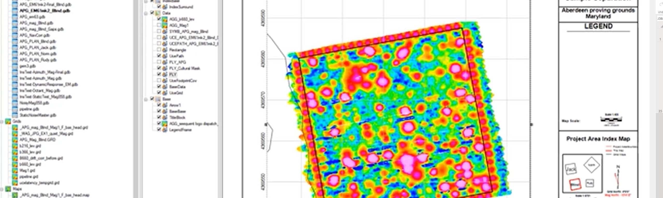
[00:28:14.880]So a few things to note

[00:28:16.010]about using the footprint coverage tool

[00:28:18.110]is that you need a polygon shape file

[00:28:21.160]or some sort of text file

[00:28:22.880]that will outline your survey area.

[00:28:25.730]So here I have my survey area outlined in black

[00:28:29.530]and that was a CSB file.

[00:28:32.630]Also here I have some cultural masks in my survey,

[00:28:36.450]so this is a polygon file supplied to me.

[00:28:39.430]And it just shows an area that could,

[00:28:41.250]that’s an exclusion zone,

[00:28:42.430]so there could be anything here that needs to be avoided.

[00:28:45.940]But this doesn’t sit inside my actual survey blocks,

[00:28:48.750]so it’s not going to really affect the footprint coverage.

[00:28:53.170]However if you do have a cultural mask in here,

[00:28:55.430]it will be taken into consideration.

[00:28:58.630]Okay, so the size of the footprint

[00:29:02.180]will depend on the sensor type

[00:29:05.370]and the type of UXO you’re looking for as well as the depth.

[00:29:12.070]So the two parameters we need are the size of our footprint

[00:29:15.840]and the polygon or shape file defining our survey boundary.

[00:29:23.250]Okay, so I’m going to jump into the tool

[00:29:25.660]which is under data preparations, QA, QC tools

[00:29:30.210]footprint coverage.

[00:29:35.999]Okay, so within the footprint coverage tool,

[00:29:39.220]I have a database that I’m with

[00:29:42.640]and I also have a survey boundary file

[00:29:45.640]which I talked about earlier

[00:29:46.920]which is the black line surrounding the survey area.

[00:29:50.860]And I’ve also input my culture mass because I have one.

[00:29:54.770]And so the footprint shape,

[00:29:56.940]this is the polygon that’s used to calculate the footprint.

[00:30:00.720]We have options here for square or circle,

[00:30:03.730]so square works good for some electromagnetic sensors

[00:30:08.030]and circle works good for magnetic sensors.

[00:30:11.390]So with this new tool,

[00:30:12.890]this allows you to calculate a more accurate

[00:30:14.760]footprint coverage for any size survey,

[00:30:17.880]for example the resolution of your circle.

[00:30:20.420]So if you reduce the resolution,

[00:30:22.830]that just means there’s a fewer points within the circle

[00:30:27.390]polygon that you used

[00:30:29.450]and this actually can speed up the process.

[00:30:32.090]So for our very large survey

[00:30:33.590]you might want to reduce the resolution of your circle.

[00:30:38.300]And finally the footprint size,

[00:30:41.330]what I talked about earlier that has to relate,

[00:30:43.480]this relates to the size of the target

[00:30:46.250]and the depth and the sensor,

[00:30:48.830]so I’m just going to use one for this survey.

[00:30:52.391]And I want to display the coverage on my current map.

[00:30:55.650]And then finally I’m going to plot my legend.

[00:30:58.450]So I want to locate that,

[00:31:01.510]you can do so by clicking locate

[00:31:04.060]and wherever you click will just be a temporary location

[00:31:08.260]’cause you’re able to move that particular legend

[00:31:12.520]item after.

[00:31:14.250]So I’ll click okay.

[00:31:17.590]And now this is calculating the footprint coverage

[00:31:20.460]and I used to circle, medium resolution,

[00:31:23.900]shouldn’t take too long.

[00:31:26.550]And I’ll update the legend,

[00:31:29.380]so I’ll say no to keeping the current legend.

[00:31:33.300]Okay, so I just put my data value here

[00:31:35.740]or my legend entry here, I’m just going to move that up here.

[00:31:42.740]That’s just a result of where I clicked my cursor.

[00:31:47.603]So this is a great tool because

[00:31:49.410]you can see here the percent covered.

[00:31:51.950]So this survey had 99.85% coverage, which is good

[00:31:57.180]and you can just make sure that you meet

[00:31:59.590]the project specifications.

[00:32:02.260]And it shows the total area covered

[00:32:04.350]and your footprint size and the polygon used.

[00:32:08.380]So if you zoom in you do see

[00:32:09.550]there’s some gaps in the survey, these white areas here.

[00:32:13.590]And it’s possible you might need to go back

[00:32:15.857]and resurvey that if you want 100% coverage.

[00:32:22.460]Now I’m going to look at targets and picking positive peak

[00:32:24.770]targets from a profile and data linking.

[00:32:34.320]So in oasis montaj we have several ways to pick targets.

[00:32:37.750]We can pick tickets from our profiles

[00:32:40.350]which I have here on the left

[00:32:42.050]or from grids which I have on the right.

[00:32:44.810]We can also do this picking manually or automatically.

[00:32:48.060]So right now I’m going to show you how to pick targets

[00:32:50.190]from profiles automatically

[00:32:53.440]and then to look and compare with what we see on our grid

[00:32:56.850]to what we see in a profile view

[00:32:59.330]and the targets that were chosen.

[00:33:01.470]And also I’m going to bring up some parameters

[00:33:03.780]within the target picking tool that are important.

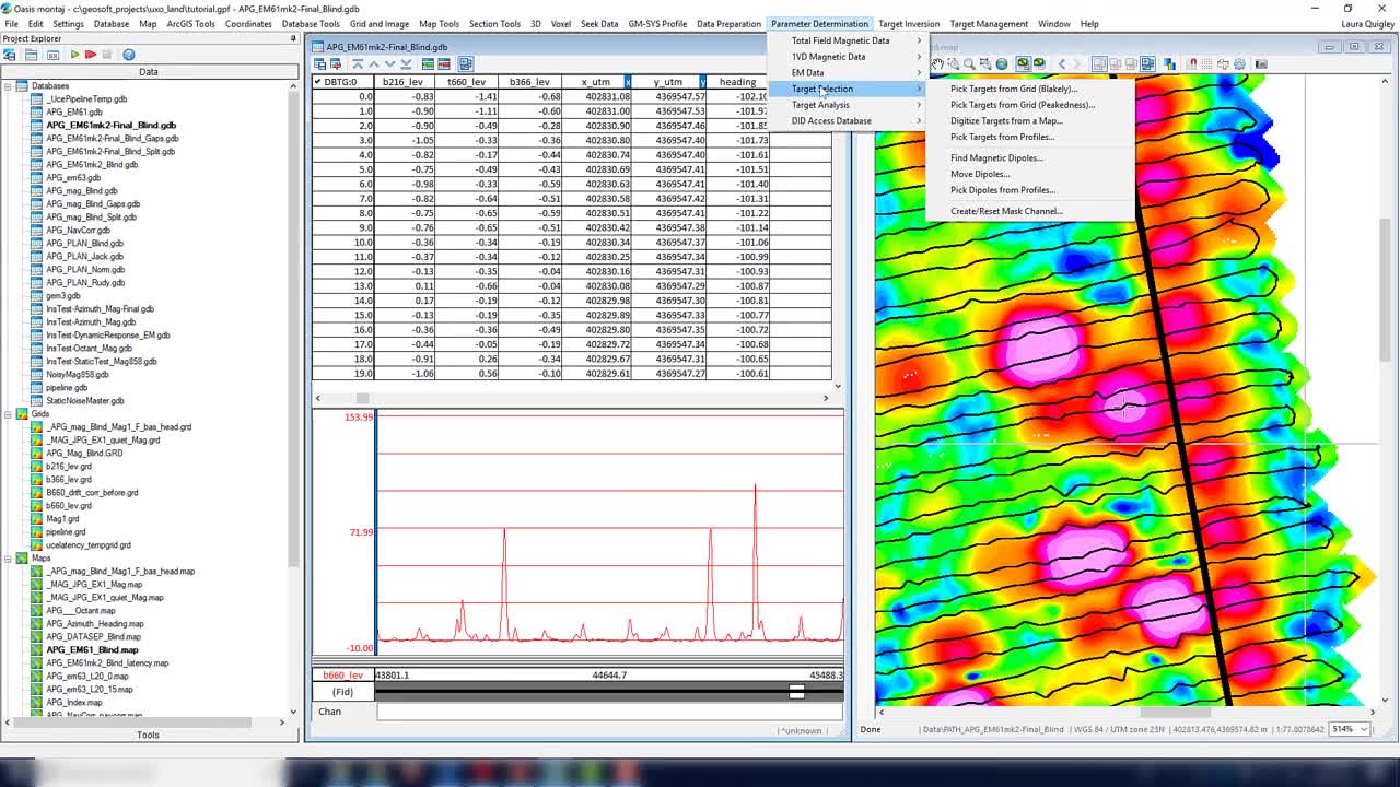
[00:33:07.500]Okay, so under perimeter determination target selection,

[00:33:13.610]we can choose pick targets from profiles.

[00:33:19.280]Okay, so I’m going to use the EM profile in the EM database,

[00:33:23.230]so this is my B660 underscored left channel displayed here,

[00:33:28.233]so this is just one of my time gates in my EM51 data.

[00:33:32.070]And the same channels also gridded here on the right

[00:33:35.370]and the survey lines are shown in black

[00:33:37.570]on the right as well.

[00:33:40.290]Okay, so in order to do target picking from profiles,

[00:33:43.073]we need to enter a few things.

[00:33:46.170]So we want to tell it the channel to choose, to pick from,

[00:33:48.660]so I’ve chosen this B660 lev.

[00:33:51.380]And a base level, so this is level data, so zero.

[00:33:54.680]And the minimum amplitude,

[00:33:55.900]so this is the threshold in which the target will be chosen.

[00:33:58.820]So anything below 25 millivolts

[00:34:01.430]will not be picked as a target.

[00:34:03.190]And so this value needs to be known beforehand

[00:34:06.270]either from a survey contractor or from other data

[00:34:08.690]in the area that you know a good value to put in here,

[00:34:12.070]so anything less than 25 will not be paid as a target.

[00:34:16.830]And this tool will also create an additional database.

[00:34:21.050]So it’ll create a target database

[00:34:23.010]and I’ve given that target database name,

[00:34:24.910]so I’ve just called it targets dot GDB.

[00:34:29.010]And within that target database, we can give it a line name,

[00:34:32.850]so within a target database a line is known as a group,

[00:34:36.680]so that’s just a good tip here to remember.

[00:34:39.830]So I’m going to call this line or group

[00:34:42.270]targets underscore profile

[00:34:44.900]to signify that I’ve picked these targets

[00:34:47.120]based on my profile.

[00:34:48.230]And that way if I add any additional targets

[00:34:50.900]or if I decide to merge some targets later,

[00:34:53.350]I can append a name to the line to signify that.

[00:34:59.890]Okay and I’m going to leave this

[00:35:00.810]additional filtering here blank for now

[00:35:02.780]and just go with target picking anything above 25.

[00:35:09.850]Okay, so we have a target database that’s created

[00:35:12.280]and within the target database,

[00:35:13.690]this can serve as a dig list or a target list.

[00:35:17.200]And it shows that there has been 99 targets

[00:35:20.620]picked along profiles, and we have an x, y target ID

[00:35:26.230]on anomaly value, we also have these channels here.

[00:35:29.850]So this shows you your within your survey database,

[00:35:32.780]the distance along line.

[00:35:34.500]So within this survey, the EM61 survey

[00:35:37.110]I have one single line, so I haven’t split my date on lines,

[00:35:40.410]so it just shows you the long line distance.

[00:35:42.697]And it also shows you the fiducial within the survey

[00:35:45.300]that, that target was chosen.

[00:35:50.220]If you have targets that have been chosen from a survey,

[00:35:52.360]which has been split on lines,

[00:35:54.060]you’ll also get a survey line channel as well

[00:35:56.460]within your target database

[00:35:58.760]and again the group or the line is shown here.

[00:36:05.960]Okay, so now I want you to display my targets on my profile,

[00:36:10.400]so I’m just going to display my map as well as my profile view.

[00:36:17.620]Also within our survey database we have two new channels.

[00:36:21.740]So these two new channels here have been added,

[00:36:24.040]so this is a target ID channel

[00:36:26.360]and this is the profile value,

[00:36:29.590]so the anomaly value of the target.

[00:36:32.160]And although they appear empty,

[00:36:33.860]if I plot the symbol of my anomaly

[00:36:39.000]and I rescale my profile I’ll see that all these anomalies

[00:36:43.240]here were picked as targets.

[00:36:45.670]Okay, so I’m just going to zoom into an area,

[00:36:47.880]so this is a fairly dense line,

[00:36:50.100]as I said they weren’t split on lines.

[00:36:53.440]Okay, so I’ve also displayed a grid

[00:36:57.450]as you can see the red horizontal lines in my profile.

[00:37:01.190]So this value is just every 25 millivolts,

[00:37:05.610]so that’s the minimum,

[00:37:06.780]this first line here would be the minimum threshold

[00:37:08.610]for a target to be chosen.

[00:37:10.490]So this is just a good way to look through your profile

[00:37:13.070]and if anything above this line was not chosen,

[00:37:16.040]you can go back in and add or delete pics.

[00:37:21.700]So next I’m going to show you how to look at these profiles

[00:37:24.350]on the gridded channel here on my map.

[00:37:28.210]So we have a data linking tool.

[00:37:31.030]So if I click on the data linking tool,

[00:37:32.850]I’m able to link my map to a survey or target database,

[00:37:39.630]my EM61 database.

[00:37:42.000]And if I click okay and then I decide to click on my map,

[00:37:46.690]I can actually find the location in my profile.

[00:37:51.680]Okay, so this comes handy when you want to see

[00:37:54.330]a target in your map and where it sits on your profile.

[00:37:59.500]So I’m going to show you a few other tips and tricks here

[00:38:02.010]and the first one is how to display your targets

[00:38:05.420]on your map.

[00:38:07.230]So in my map manager,

[00:38:09.430]I’ll just pin this open so we can take a look.

[00:38:12.790]So important things to note here when linking your profile

[00:38:16.020]data or your database data to a map

[00:38:18.750]is that you need to have a path of that database

[00:38:21.290]on your manager.

[00:38:22.700]You don’t necessarily have to have it turned off,

[00:38:24.530]so I have mine displayed here, the black lines.

[00:38:27.720]I can turn it off and still link my map to my database.

[00:38:31.590]However, it needs to be at least

[00:38:33.370]in my map manager to do that

[00:38:35.590]’cause when you click on this data linking tool

[00:38:37.370]it searches for that particular database.

[00:38:41.040]Okay, so I clicked that

[00:38:43.400]and like I said, you can click anywhere on your map

[00:38:45.960]and that’ll go to that position in your database

[00:38:48.460]and on your profile.

[00:38:50.680]So I’m going to display my symbols on my map,

[00:38:54.200]so I’m going to select my target database,

[00:39:00.080]simply double click.

[00:39:04.050]And then I would like to put a symbol plot on my maps,

[00:39:06.630]under maps tools, symbols, location, plot.

[00:39:11.640]And then I can choose my single, so I’ll use x’s,

[00:39:15.180]I’ll make them 1.5 millimeters

[00:39:16.850]and I’ll put black as the color.

[00:39:20.440]Okay, so now we can see if I zoom into my map,

[00:39:23.160]all my targets from my target database

[00:39:25.360]had been plotted on my map.

[00:39:27.940]And again I’ll just go back to looking at the database

[00:39:30.590]along with the map.

[00:39:32.550]So in order to look at this target,

[00:39:34.590]say this one here in my database,

[00:39:36.540]I will turn away data linking tool,

[00:39:39.690]I’ll select my survey database.

[00:39:46.330]I will also select the pen to cursor on all maps,

[00:39:50.120]so that allows the data linking to go both ways.

[00:39:53.520]So for example if I want to see where this profile

[00:39:55.860]or this target sits, I click on that

[00:40:02.890]and it takes me to that position in my map.

[00:40:14.650]Okay, so this is a great tool to use,

[00:40:16.530]if you see anything you’d like to add

[00:40:18.530]from your profile or from your map.

[00:40:22.730]So this target here for this anomaly here for example,

[00:40:26.490]you can see it’s just below the threshold of 25.

[00:40:29.430]However who might want to go back in

[00:40:31.110]and add that for some reason.

[00:40:34.900]Now we are going to look at managing our targets,

[00:40:36.790]so adding and merging targets.

[00:40:41.290]Okay, so now I want to talk about some tips and tricks

[00:40:43.610]and just show you how to add and merge targets,

[00:40:47.060]so this is a target management workflow

[00:40:49.840]we’re going to go through.

[00:40:52.030]I’m going to add targets based on my profile view

[00:40:54.330]which I have here in my bottom left corner.

[00:40:59.290]First of all I’m going to zoom into an area

[00:41:03.210]that I’d like to add a target to.

[00:41:06.920]So I see this peak here and I, for some reason,

[00:41:09.840]would like to add that to my target list,

[00:41:12.110]whether it’s close enough to my threshold

[00:41:14.470]or have additional information that tells me

[00:41:16.130]this should be picked as a target.

[00:41:18.860]Okay, so in order to add targets,

[00:41:21.380]you can simply right click on your profile view

[00:41:24.460]and you’ll have these UXO land options here at the bottom.

[00:41:28.310]So these options here will only be available

[00:41:30.970]when you have your UXO land menus loaded on the top.

[00:41:35.200]So first of all I’ll just show you how to configure

[00:41:37.450]some of the settings.

[00:41:39.410]So they’re very similar to the automatic picking,

[00:41:42.660]we are going to use our database with our EM data

[00:41:45.760]as the survey database,

[00:41:47.190]so that’s this profile view I have on my left.

[00:41:51.280]And I’m going to snap to the closest peak,

[00:41:53.380]so remember I picked my target it’ll snap to that peak.

[00:41:58.200]And I’m going to include my new target in my target’s database,

[00:42:00.940]so I won’t create a new database.

[00:42:02.800]But I’m going to create a new group, so a new line.

[00:42:09.860]It’ll just show you the additional target

[00:42:11.700]in that line or group.

[00:42:13.490]You don’t have to create a new group,

[00:42:14.720]you can just simply add to your targets profile group.

[00:42:17.640]But I’m just going to create an another group

[00:42:19.500]just to show you how that works.

[00:42:22.050]Okay and then I click okay, so that’s just my settings.

[00:42:26.520]Now I want to add a target, so I want to add this target here,

[00:42:29.767]I’m just going to zoom it a bit more.

[00:42:33.620]And to add the target I simply left mouse click,

[00:42:37.590]so it’s highlighted in my profile and my database

[00:42:41.840]and then I’m going to right mouse click

[00:42:43.910]and select add target.

[00:42:47.380]Okay, so there’s a target added

[00:42:49.650]since I created a new line or group in my target database

[00:42:54.220]I end up with two new lines or two new channels

[00:42:57.390]in my target database, so these are my additional targets.

[00:43:01.440]So I’m going to display that profile as a symbol.

[00:43:07.960]So I click anywhere in my channel and click show symbols.

[00:43:13.290]So now you see that this is a new target,

[00:43:17.050]it’s also in my target database in a new line,

[00:43:21.250]so I’ve created a new line with my additional targets.

[00:43:26.280]And like I said

[00:43:27.113]you could have added that target to this list,

[00:43:29.420]so there’s two options.

[00:43:31.730]And I’m going to rescale all and you can see my original

[00:43:35.410]automatic picked targets and my manually picked target.

[00:43:41.270]Okay, so now I want to show you how to merge targets.

[00:43:44.930]So I’m going to jump over to the map and I’m going to

[00:43:49.290]open this and zoom into an area where

[00:43:52.370]I might consider two targets are one

[00:43:56.320]or multiple targets or just one.

[00:44:02.000]I do that and I’m going to just focus on my EM database

[00:44:07.660]and my map.

[00:44:15.670]Okay, so I’m going to focus on these two targets here,

[00:44:20.970]I’d like to merge them.

[00:44:28.160]Yeah, so this one and this one.

[00:44:36.430]So I’m going to zoom in on my profile view,

[00:44:40.280]this is just a good way to visualize it as well.

[00:44:44.960]However if I had split my data on lines,

[00:44:47.800]I might see that this is the same target

[00:44:50.570]on two separate lines,

[00:44:51.930]but since I’m working with one line in my EM database,

[00:44:55.280]it’s kind of hard to make that call based on

[00:44:58.840]what line this is on, however I can also plot my path.

[00:45:05.910]So under target management,

[00:45:09.160]target list management merged targets.

[00:45:18.380]Okay, so the important thing to note

[00:45:19.960]is whenever you’re emerging targets,

[00:45:21.570]you want to pick your new location accurately

[00:45:24.950]and we have several options to do that.

[00:45:27.340]We put our target database as the targets database

[00:45:31.210]and the input group I will use profiles, targets profiles

[00:45:35.640]’cause that’s where my targets that I’d like to merge are.

[00:45:38.740]And I’m going to use the same data channel

[00:45:40.730]I’ve used the whole time to pick my targets.

[00:45:44.380]Here we have two options, we can choose a radius,

[00:45:47.260]so you merge all targets within a given radius

[00:45:49.900]of where you choose or polygon.

[00:45:53.010]So I like to use polygon,

[00:45:54.230]it’s simple and easy just to draw a polygon around a group

[00:45:57.710]of targets that you’d like to merge.

[00:46:00.600]Okay, so where we locate our target is chosen here.

[00:46:04.400]So centroid location is simply the average

[00:46:07.720]of the individual target locations.

[00:46:10.570]So it just takes an average

[00:46:12.240]and put your new target in that position.

[00:46:17.580]So the maximum peak location is just simply

[00:46:19.900]the location of the individual target

[00:46:21.700]with the highest value, so that’ll be your new target.

[00:46:25.180]And finally we have weighted average.

[00:46:28.090]So the centroid of the individual targets

[00:46:30.180]weighted by their anomaly value.

[00:46:33.210]So this means the new target location will be closer

[00:46:36.060]to the larger of the individual target.

[00:46:39.290]So I’m going to show you a couple of these tools

[00:46:41.910]in slightly different results.

[00:46:45.600]So I’ll start with the center, so the average location.

[00:46:49.360]Okay, so for the value of the target,

[00:46:51.080]we can either use the average of all the targets,

[00:46:53.840]the grid value at the location of our new target

[00:46:56.840]or the maximum of all the targets

[00:46:58.670]that we have chosen to merge.

[00:47:00.220]So this value here, grid value of the location,

[00:47:02.910]that could be a value of your EM in between lines,

[00:47:06.280]’cause grids are just simply interpolated between lines.

[00:47:09.460]Right now all our targets sit on lines

[00:47:11.250]’cause they were picked from profiles.

[00:47:13.500]So if I merge these three targets for example

[00:47:16.300]and I choose this option

[00:47:18.320]and the location happens to be here,

[00:47:20.580]that’ll be the value of my new target.

[00:47:23.330]So my new target line or group,

[00:47:25.500]I will call targets profile merged average.

[00:47:29.770]And again I’ll give it the survey database name

[00:47:31.960]and this’ll put two new channels in my survey database

[00:47:34.740]associated with this target line.

[00:47:42.140]And then I’m going to choose some symbols,

[00:47:44.720]so I’m going to use the triangle and I’m going to use this color

[00:47:48.220]and then I’m going to go back in and run this again

[00:47:49.890]and just show you how the targets look

[00:47:52.350]with a different location option.

[00:47:56.830]So if I click okay and then I begin to draw my polygon.

[00:48:01.050]So I’ll pick these guys here just ’cause there’s three.

[00:48:05.460]So you don’t have to click a lot,

[00:48:06.740]you can be very rough and when you’re done,

[00:48:09.900]right button click and select done.

[00:48:13.390]Okay, so now this has given me a new target.

[00:48:22.960]Okay, so it’s merged these three targets into one

[00:48:26.380]and in my target database, I will have a new group.

[00:48:33.540]And this has included all the targets that are merged.

[00:48:37.300]So essentially it took my old target group,

[00:48:41.420]kept those as they were.

[00:48:44.800]So it merged these three

[00:48:46.010]and there’ll be two less in my new group.

[00:48:49.240]Also my survey database I have two new lines

[00:48:52.100]and they’re associated with the merge targets.

[00:48:58.220]Okay, so now if I run that tool again.

[00:49:08.760]And say I use maximum peak location,

[00:49:14.310]I’ll simply change my symbol to a green triangle

[00:49:20.360]and I’ll just put underscore two here.

[00:49:23.900]So don’t want to overwrite that,

[00:49:25.350]I want to see both options on my map.

[00:49:30.970]Okay and then I’ll do the same,

[00:49:34.390]my input group is the original target profile group.

[00:49:43.570]Okay.

[00:49:46.690]And that just tells me that I’ve merged from 100

[00:49:50.890]and now I have 98 targets,

[00:49:52.330]I’ve merged three targets into one.

[00:49:56.170]So if you seen the map manager, I have two symbols.

[00:50:06.170]So here’s the difference in the location,

[00:50:08.840]so the first one I chose to use the average,

[00:50:11.230]the second one I said put my new target on the maximum peak.

[00:50:15.950]Okay, so the tip here is mainly just to be aware

[00:50:19.300]that these options exist

[00:50:20.640]and how they will change the location of your new target

[00:50:23.350]from a group of targets that have been merged

[00:50:25.770]and also how they will affect

[00:50:27.100]the anomaly value of your new target,

[00:50:29.580]whether it be a weighted average, an average

[00:50:32.920]or simply the largest anomaly in the group.

[00:50:38.510]Next we’re going to look at picking positive peak targets

[00:50:40.950]from a grid using the Blakely method.

[00:50:48.360]Okay, so next I want to talk about how to pick targets

[00:50:50.910]based on your grid.

[00:50:57.310]So under perimeter determination, target selections

[00:51:01.100]pick targets from grid Blakely.

[00:51:05.880]Okay, so this is going to look for the positive peaks

[00:51:08.180]in our EM database

[00:51:10.370]and the input grid will be my 660 channel.

[00:51:15.180]And the level of peak detection is normal,

[00:51:17.520]so that just means it looks for a peak in four directions.

[00:51:21.940]I’m going to use the same grid value cutoff of 25

[00:51:26.140]and I’m also going to keep the same target database,

[00:51:28.360]but just add a new group,

[00:51:29.950]so I’ve added an underscore Blakely.

[00:51:34.250]And then finally I give it the survey database

[00:51:36.250]so they can add two new channels to that database.

[00:51:40.460]Okay and those two new channels are going to be

[00:51:42.130]one with the target amplitude and one with the target ID.

[00:51:51.280]And then I will choose a different color

[00:51:53.930]for my targets so I can compare with my profile targets,

[00:51:56.840]so I just chose red.

[00:52:00.190]I click okay.

[00:52:02.370]Okay, you see some targets now that have been added

[00:52:05.760]and these targets, there’s not as many that have been chosen

[00:52:09.860]through the grid option.

[00:52:11.930]And that just has to do with the parameters

[00:52:14.580]that we’ve chosen.

[00:52:15.470]So the level of detection, as well as the minimum threshold.

[00:52:21.450]So as you see there’s one target chosen here

[00:52:24.380]where if I use my profiles

[00:52:25.610]that actually picks the target three times.

[00:52:27.880]So this is a good way to compare

[00:52:29.530]and then you can investigate

[00:52:31.020]which of these options you would like to use, okay.

[00:52:33.620]So in my database I now also have two new channels,

[00:52:37.140]so these are targets Blakely

[00:52:40.200]and I can plot those as symbols as well.

[00:52:47.070]Now I’m going to talk about picking magnetic dipole targets

[00:52:49.770]from your grid.

[00:52:56.200]Okay, so now I’m going to talk about

[00:52:57.450]how you can pick magnetic dipoles as targets,

[00:53:01.430]so I’m going to show you two methods.

[00:53:03.000]We can use a grid to pick our dipoles

[00:53:05.730]or we can use a survey database

[00:53:08.300]and sometimes you might want to use both

[00:53:09.910]just to compare results.

[00:53:12.410]So first of all I’ll talk about the gridding

[00:53:14.850]and anytime we pick from a grid,

[00:53:16.610]we have to make note that the grading parameters

[00:53:19.660]that we have chosen to create the grid,

[00:53:21.440]so I’ve used a minimum curvature here

[00:53:23.600]with various parameters for my cell size,

[00:53:25.590]blinking distance, etc.

[00:53:27.490]Those gritting parameters will affect

[00:53:30.765]what dipoles are picked

[00:53:32.720]and that’s just something to make note of.

[00:53:35.210]Okay, so I’m going to go to parameter determination,

[00:53:38.860]target selection, find magnetic dipoles.

[00:53:43.440]So we’re using the grid first.

[00:53:47.010]So my input grid is mag one,

[00:53:48.420]so I’ve just created the first magnetics channel

[00:53:50.140]for this example and the minimum positive peak value,

[00:53:54.010]so that’s your threshold value.

[00:53:55.830]You want to look for anything, I’ve chosen 50,

[00:53:59.030]so I want to look for anything above 50, 50 nanoteslas,

[00:54:03.080]so that’ll be considered a target

[00:54:05.420]and the maximum dipole separation that’s in meters.

[00:54:09.320]So it’s a search radius essentially,

[00:54:11.330]so anything from your positive peak,

[00:54:13.800]that’s two meters in diameter.

[00:54:16.330]That’s a negative peak, it’ll form a dipole.

[00:54:19.800]Okay, so these two parameters here

[00:54:22.160]and I’m going to output my targets to the same database,

[00:54:24.950]target database is always

[00:54:26.930]and I’m going to create a new group within my database,

[00:54:29.460]so I’m just going to put a mag one underscore grid,

[00:54:36.550]just to note that I’ve got,

[00:54:38.430]picked these targets from a grid.

[00:54:41.440]And a new channel will be created called dipole amp,

[00:54:44.900]so that’s going to be the separation in nanoteslas

[00:54:47.900]between my negative and positive peak on my dipole.

[00:54:51.900]And finally I’m going to use my survey database

[00:54:55.160]which is mag underscore blind.

[00:54:59.000]And I’ll get to new channels in my database

[00:55:01.670]as well as new line in my target database or a new group.

[00:55:06.920]Okay and these symbols here, I’ll just leave the default,

[00:55:09.130]so these symbols are going to be a bit different

[00:55:10.900]than they were for the Blakely picking method.

[00:55:14.650]So I’ll click okay.

[00:55:24.780]Okay so these are my new targets picked from this grid,

[00:55:27.950]so you can see some dipoles were chosen here.

[00:55:31.869]And in my map these symbols to new groups here

[00:55:35.770]are the symbols for the dipole, so one is the line

[00:55:39.160]and the other portion of the symbol is the actual x’s

[00:55:42.750]that joined the positive and negative peak.

[00:55:46.400]Probably want to talk about picking magnetic dipole targets

[00:55:48.970]using your profile data.

[00:55:52.120]Perimeter determination, target selection,

[00:55:55.500]pick dipoles from profile.

[00:56:00.070]Okay so this is a similar dialogue,

[00:56:02.370]we’re going to use our mag database and selected lines,

[00:56:06.120]I’ve outlined selected.

[00:56:08.720]I’m going to pick my anomalies from my mag one channel,

[00:56:15.580]the same one I used to grid my data.

[00:56:19.690]And again I’ll use the same minimum threshold

[00:56:22.210]and dipole separation.

[00:56:24.420]I’m going to, I’ll put the targets to my target database

[00:56:28.270]and I will call this group mag one profile.

[00:56:34.690]And I can leave this here as the default,

[00:56:38.230]so this is going to be my new channel that’s created

[00:56:42.210]from this group and I’ll click okay.

[00:56:51.710]Okay, so I’m going to turn off my previous pics

[00:56:55.100]and we see we have some additional pics

[00:56:58.860]from using the profile.

[00:57:01.660]Okay, so now I want to just look at the database

[00:57:05.980]and see what my targets look like.

[00:57:09.850]So in the survey database,

[00:57:12.280]we will have additional target channels.

[00:57:18.290]So again we have a target ID

[00:57:21.560]and we have a anomaly amplitude,

[00:57:24.580]so I’m going to plot the amplitude.

[00:57:36.160]Okay and if you scroll through the lines

[00:57:37.840]you can look at the difference

[00:57:38.980]between the targets you’ve picked from the grid

[00:57:41.560]and the targets you picked using the profile method.

[00:57:48.380]So in today’s webinar, we’ve covered

[00:57:50.180]the UXO land workflow overview

[00:57:52.550]and the associated learning path.

[00:57:55.570]We’ve looked at forward modeling target anomalies,

[00:57:58.620]applying heading corrections using instrument tests,

[00:58:02.750]calculating the footprint coverage,

[00:58:05.410]picking targets from peaks on your profile and data linking.

[00:58:09.730]Adding and merging those targets.

[00:58:12.680]Picking targets from a grid using the Blakely method.

[00:58:16.660]Finally, we looked at magnetic dipoles

[00:58:18.340]and how we could pick targets using the dipoles

[00:58:20.450]from either a grid or profile.

[00:58:24.290]I want to thank everyone for joining me today

[00:58:25.930]and I hope everyone got something from this webinar

[00:58:27.940]that they’ll find useful to help them

[00:58:29.690]with their UXO land workflow.