Industrial Minerals: How to predict material quality faster and more accurately

This webinar will provide an overview of Seequent solutions in the Industrial Minerals market that can help you more accurately and quickly predict material quality to better inform mine planning and other areas of Industrial Minerals operations.

This webinar covers the following:

• An overview of common challenges faced by the Industrial Minerals Mining Industry
• How to overcome these challenges to reduce waste and improve quality of stock
• A customer success story -Lhoist
• Presentation an innovative workflow for IM industry using collaborative tools and technology

Overview

Video Transcript

[00:00:02.370]<v James>Okay, welcome again,</v>

[00:00:03.560]once again to today’s webinar.

[00:00:05.750]So my name is James Edwards

[00:00:07.300]and I’ll be running the webinar for today.

[00:00:09.400]Although my title is Business Development Manager

[00:00:11.630]for the Industrial Mineral Sector,

[00:00:13.160]my background is actually is a geologist.

[00:00:15.170]My main focus being on Exploration and Resource Estimation.

[00:00:19.454]And basically today,

[00:00:20.287]we’re going to be introducing Seequent as a company

[00:00:22.340]and discussing how we support our clients

[00:00:24.190]to address some of the common technical challenges

[00:00:26.360]we find in the Industrial Minerals Industry.

[00:00:29.480]The second half of the presentation

[00:00:30.670]will be a live demonstration of our products.

[00:00:32.400]And It’s going to help you to understand the concepts

[00:00:34.880]that we’re discussing today.

[00:00:37.110]So let’s get started.

[00:00:40.000]So who are we?

[00:00:41.470]Some of you may have heard of Seequent.

[00:00:42.970]Others may be more familiar with the name of our products,

[00:00:44.880]such as Leapfrog Geo.

[00:00:46.890]In essence, we’re a software company,

[00:00:48.730]but where we differ is that from the very beginning,

[00:00:50.570]we’ve understood that the context

[00:00:52.370]is the key to connecting the right information,

[00:00:54.400]give us the right insights to make the right decisions.

[00:00:58.000]Our vision is to enable better decisions

[00:00:59.670]about earth, environment and energy challenges.

[00:01:03.510]We find our customers are tucked

[00:01:04.670]in some of the world’s most challenging problems

[00:01:06.220]using not just our software,

[00:01:08.100]but also the technical advice and expertise our global team

[00:01:10.580]of industry experts can provide.

[00:01:13.690]Above all we believe in constant innovation

[00:01:15.960]by thrusts and the businesses we support.

[00:01:19.280]By working in partnership,

[00:01:21.020]we ensure we stay at the forefront of innovation

[00:01:23.140]and consistently add value back

[00:01:24.520]into the work our clients undertake.

[00:01:31.380]So I’m not trying to state the obvious

[00:01:32.410]for those in the pool,

[00:01:34.230]but we do understand that the Industrial minerals sector

[00:01:36.380]can often be misperceived or misunderstood.

[00:01:39.200]People really understand,

[00:01:40.210]or at least underestimate the multiple uses and requirements

[00:01:42.910]of markets for industrial minerals.

[00:01:45.090]By quality control and production, product consistency,

[00:01:48.000]and customer relationships are paramount

[00:01:49.830]to ensure sustainable profitable business.

[00:01:53.270]The market is driven by the market

[00:01:54.480]therefore product quality, consistency is essential

[00:01:56.841]and drives acceptance.

[00:01:59.140]Equally, funneling the demand

[00:02:00.510]requires building customer relationships

[00:02:02.700]which are formed on credibility, reliability,

[00:02:04.880]and mutual support.

[00:02:06.999]Probably shouldn’t underestimate in the current climate

[00:02:09.410]obtaining a license to operate

[00:02:10.660]from local communities will become a bigger issue.

[00:02:13.610]Having the right tools to communicate and share information

[00:02:15.880]will support community relationships and building.

[00:02:28.190]So how easy would life be

[00:02:29.180]if you knew exactly what was in the ground

[00:02:31.070]and exactly where it was?

[00:02:33.670]Now while we might never be able to achieve exactly that.

[00:02:36.790]What we typically find at the moment is that the journey

[00:02:38.610]of developing resource insight from exploration

[00:02:40.730]through to short term mind planning

[00:02:42.550]is often scattered across organizational boundaries,

[00:02:45.120]different data sources and different geological models.

[00:02:49.410]We see processes and procedures at one site

[00:02:51.640]could often be in complete contrast to another.

[00:02:54.600]And not only is this lack of standardization drive

[00:02:56.620]inefficiencies in your business

[00:02:58.360]where best practice does exist is often not recognized

[00:03:01.659]and therefore isn’t shared across the company.

[00:03:05.390]Are you working in an industry that is as market

[00:03:06.920]and customer driven as yours,

[00:03:08.400]you obviously need to be reactive to change in demand.

[00:03:11.190]Contracts are specific and relationships are built

[00:03:13.180]on the reliable supply of material to meet customer needs.

[00:03:16.690]So how quickly can you currently react

[00:03:18.660]and how much certainty do you have in those decisions?

[00:03:21.610]You can’t change the natural variability of a deposit

[00:03:24.170]by increasing the knowledge of your resource base.

[00:03:26.430]You can reduce uncertainty

[00:03:28.130]and move forward with greater confidence.

[00:03:31.368]With greater confidence

[00:03:33.660]you can get an improved understanding of your resources.

[00:03:36.880]For example, with a better understanding,

[00:03:38.930]can you help to redefine waste to something more marketable?

[00:03:41.737]And potentially with less waste obviously

[00:03:43.650]it would drive down operational costs.

[00:03:49.170]So what do we offer?

[00:03:51.748]We’ll take a look at what Seequent has,

[00:03:53.030]and then we’ll say how we believe we can support

[00:03:54.870]your business to extract maximum value from the resources

[00:03:58.020]you have and address the challenges within the industry.

[00:04:01.373]So Seequent currently offers solutions to several industries

[00:04:04.320]that whilst diverse all gain value from a greater insight

[00:04:07.080]into what is below the ground.

[00:04:09.650]For the industrial metals sector our mining

[00:04:11.300]product suite covers all aspects of the exploration

[00:04:13.840]and mine life cycle.

[00:04:15.750]The products are focused around

[00:04:16.647]our Central data management platform.

[00:04:19.320]So Central helps you visualize track

[00:04:21.140]and manage your geological data from a Centralized

[00:04:23.310]or comfortable environment.

[00:04:24.910]It brings project teams together, helps stay connected

[00:04:27.680]and enables your team to make confident decisions

[00:04:29.480]when it matters the most.

[00:04:32.030]The policy is the only true software

[00:04:32.863]as a solution of its kind,

[00:04:34.590]offering affordability and flexibility.

[00:04:37.160]It comes with both mobile and web based login

[00:04:40.690]and data management tools with on the spot validation.

[00:04:43.680]So anywhere that you’re drilling or collecting samples,

[00:04:45.490]then deposit can make the process easier for you.

[00:04:49.030]Leapfrog sets a standard in geological modeling

[00:04:51.070]and reduces risk by creating more time

[00:04:52.850]and opportunity to understand the geology.

[00:04:55.480]Leapfrog Geo is our flagship application,

[00:04:57.370]which harnesses the power of implicit modeling to build

[00:04:59.920]and update models significantly faster

[00:05:02.730]and integrated with Geo

[00:05:03.700]is our estimation software package, EDGE.

[00:05:08.130]So EDGE is a natural progression

[00:05:09.390]from GIS traditional Geological modeling

[00:05:11.230]into the resource estimation space.

[00:05:14.060]We find what EDGE is used to gain

[00:05:15.150]a relief from Geo, to solution manage, robust understanding

[00:05:17.790]of the geology with sound resource domain,

[00:05:20.070]and defensible variography and estimates.

[00:05:23.410]We also have GSS technology platform,

[00:05:25.410]which is an industry standard within the geosciences.

[00:05:28.505]Within JSF packages target for our GIS software is regarded

[00:05:31.960]as the market leader in geological application for Esri.

[00:05:34.080]So it delivers essential workflows for geosciences

[00:05:36.930]and GIS professionals working in the ArcGIS platform.

[00:05:40.950]And lastly Geoslope provides geotechnical

[00:05:43.060]and environmental engineers

[00:05:43.970]with rigorous analytical capability

[00:05:46.020]to solve diverse geotechnical and geoscience problems.

[00:05:49.590]Geoslope helps users work across a broad range

[00:05:52.030]of engineering use cases,

[00:05:53.270]including excavations and open pit mining.

[00:06:00.100]So how are we different?

[00:06:02.410]Depending on your size, complexity and need,

[00:06:04.090]there’s a combination of products that will enable you

[00:06:05.900]to extract maximum value from your data.

[00:06:09.130]The integrated nature of our products and ease of use

[00:06:10.980]will help break down barriers across your operations.

[00:06:13.950]The software doesn’t require years of experience

[00:06:16.140]to drive the desired result.

[00:06:17.990]It follows a logical workflow, that’s has been designed

[00:06:20.650]by geologists and in partnership

[00:06:21.920]with major industry clients.

[00:06:25.060]A Central platform,

[00:06:26.810]which we’re going to have a look at in the demonstration

[00:06:29.220]provides a collaborative and connected environments.

[00:06:32.750]Before Central, we found that the majority of our customers

[00:06:35.280]would use PDFs, PowerPoints or print outs to try

[00:06:38.010]and convey key information about their models.

[00:06:40.600]Often impacts of changes would be discussed by moving

[00:06:43.090]between different bits of paper.

[00:06:46.900]With Central they have these discussions

[00:06:48.370]around the data in 3D.

[00:06:50.530]Even if remotely, they can have it between sites and office

[00:06:53.280]via the online platform.

[00:06:55.890]Opinions, decisions and knowledge can be captured in 3D

[00:06:58.600]and preserved for future consideration.

[00:07:01.120]Central also helps drive standardization

[00:07:03.430]and it shows data is secure, available and auditable.

[00:07:07.530]Our implicit modern engine and dynamic updating

[00:07:09.670]enables you to update your models in hours

[00:07:11.400]rather than weeks.

[00:07:13.410]We also have clients, one of our clients for example,

[00:07:15.410]has over a thousand things in their model.

[00:07:18.030]And we found updates for limited to at least once a year

[00:07:20.490]and no sooner had one resource model been completed,

[00:07:22.820]the next one would start.

[00:07:24.750]With Leapfrog Geo they can now incorporate new data

[00:07:26.860]on a weekly basis.

[00:07:28.500]Through this they can adjust their short term plan

[00:07:30.210]to account for changes in the resource base,

[00:07:32.350]ensuring that they’re extracting maximum value

[00:07:34.520]from what’s in the ground.

[00:07:38.440]And so being able to update your models rapidly presents

[00:07:41.590]the opportunity to work differently.

[00:07:44.800]If inclusion of data isn’t your bottleneck,

[00:07:47.180]can you sample more frequently.

[00:07:49.990]Could trail campaigns be executed differently?

[00:07:52.250]Could areas of risk be mattered, be managed smarter.

[00:07:58.280]Our products will help you better define the chemical and

[00:08:00.320]physical characteristics of your deposit.

[00:08:02.530]The integration of geological information into one better

[00:08:04.850]universal source of truth helps optimize operations,

[00:08:08.210]create an executable mind plan

[00:08:09.910]and avoid quality issues at the source.

[00:08:12.450]And with the insight gained from having the latest

[00:08:13.923]data available to you,

[00:08:15.390]your model can move from reactive to proactive

[00:08:17.990]and being proactive allows you to combine

[00:08:19.830]business strategy with resource knowledge

[00:08:21.910]and deliver a high quality consistent product

[00:08:23.940]for your customer base.

[00:08:29.110]And one of the best cases or examples we have.

[00:08:31.600]I don’t know if you’ve seen the latest case study

[00:08:33.530]it’s been sent out some of the material

[00:08:35.530]we’ve distributed recently.

[00:08:37.350]Our lawyers to a great example were using our products

[00:08:39.410]as driven collaboration across technical teams

[00:08:41.860]and radically improved their workflows.

[00:08:44.560]They’ve moved from a reactive model,

[00:08:45.930]to one where data is incorporated into the model

[00:08:47.930]on a daily basis.

[00:08:49.600]And this provides the lawyers with a predictability

[00:08:51.430]of impurities and contaminants before they blast.

[00:08:56.190]What they found is the ability to know exactly

[00:08:57.870]what they can supply to customers,

[00:08:59.410]puts their business in a position of strength.

[00:09:02.110]So to know exact quality at specific locations

[00:09:04.790]in the quarry, allow them to plan to ensure that

[00:09:06.640]they meet the needs of their customers.

[00:09:08.600]And with more confidence in their data,

[00:09:10.600]it provides agility and decision-making.

[00:09:15.680]Oh yeah, an easy way to explain this is a short

[00:09:18.220]30 second clip, that we made in partnership with Lhoist.

[00:09:24.108](bright upbeat music)

[00:09:29.367]<v Seequent Client>The company is motivated</v>

[00:09:31.100]to introduce innovation that keep us

[00:09:33.400]as efficient and sustainable as possible.

[00:09:35.840]And it was this motivation that led us to Seequent.

[00:09:38.240]By working together, we’ve been able to radically improve

[00:09:41.410]our workflow, to enable a much richer relationship

[00:09:44.540]with our geology.

[00:09:46.390]<v ->[Seequent Client 2] We have more confidence in our data</v>

[00:09:48.170]and it gives us agility in decision-making and ultimately

[00:09:51.830]enables us to update our model far more frequently.

[00:09:54.656](bright upbeat music)

[00:10:02.680]<v James>So you’ve heard me use the term Implicit model</v>

[00:10:03.917]in the RBF functions a few times.

[00:10:06.659]For those who are not familiar with these terms,

[00:10:09.000]I’ll have try providing a brief overview.

[00:10:12.160]But again, what you embrace in the demonstration

[00:10:13.990]will help make a lot more sense.

[00:10:19.000]So in the implicit world, one of the fundamental changes

[00:10:20.990]is we don’t just wireframe

[00:10:22.430]and force a model into our interpretation.

[00:10:25.070]We work with the data to make the best decision possible

[00:10:27.570]using both statistics and geological expertise.

[00:10:31.250]Sort of I’ll try and start by explaining the fundamental

[00:10:33.020]differences between the two methods.

[00:10:35.660]And first off, we look at the explicit method further.

[00:10:39.650]So quite frequently and modeler in an explicit software

[00:10:41.690]program is hit by several major challenges.

[00:10:44.490]One for example is the expensive software packages

[00:10:46.720]are not particularly intuitive and it can take years

[00:10:48.640]to become true to profession.

[00:10:51.170]Commonly the geologist has to work in a 2D environment

[00:10:53.520]where data is heavily restricted to sections

[00:10:55.630]and it’s up to the modeler’s expertise

[00:10:57.710]to interpret how that data was connected

[00:10:59.057]and the black spaces in between.

[00:11:02.110]For anyone not knowing what wireframing is

[00:11:04.020]modeling has to go through a painstaking exercise

[00:11:06.500]of digitizing every single point,

[00:11:08.400]and then they need to connect each of them via strings.

[00:11:11.650]These strings then sit on sections,

[00:11:13.110]which in turn are then connected into 3D space

[00:11:15.430]to create a volume.

[00:11:17.620]This exercise has to be carried out for each

[00:11:18.947]different unit and the model has to make sure that

[00:11:21.740]each volume fits the next one perfectly

[00:11:23.790]to create an air tight model without intersections.

[00:11:27.510]I’m trying to imagine what happens once new data

[00:11:28.680]is added in that model.

[00:11:30.840]The whole process of digitizing and local section

[00:11:33.150]interpretation starts over and not just for that one volume,

[00:11:36.830]but for all of the adjoining ones as well.

[00:11:39.410]And this of course results in just a ton of extra work.

[00:11:43.820]So from this perspective, it’s not surprising.

[00:11:45.390]And explicitly drive models tend to contain only one level

[00:11:48.100]of geological interpretation that may or may not respect

[00:11:50.840]other collected drill hole data,

[00:11:52.450]such as structural, geochemical or geophysical measurements.

[00:11:58.440]Now implicit software takes a completely

[00:12:00.040]different approach to 3D modeling.

[00:12:01.520]That’s just based on the mathematical evaluation of data

[00:12:03.810]in combination with skilled interpretation.

[00:12:07.040]Key to this is you have full control to make the changes

[00:12:08.990]necessary to develop a true geological interpretation

[00:12:11.920]that also takes advantage of

[00:12:13.120]a statistically sound based model.

[00:12:15.593]And the great news is that it won’t take long to learn

[00:12:17.240]as the software is intuitive and is created

[00:12:19.330]by geologists for geologists.

[00:12:22.120]In addition it allows you to integrate the more than one

[00:12:24.100]data set and quickly develop several levels of

[00:12:26.240]interpretation within one project.

[00:12:29.840]Pretty best of all is whenever there’s a new stream

[00:12:31.570]of data coming in the dynamic link between the data source

[00:12:34.340]and the final model allows for your interpretations

[00:12:36.620]to be updated almost instantly

[00:12:38.430]without the painstaking process

[00:12:39.690]of digitizing every new data point.

[00:12:43.140]Therefore, because of the way the software is set up,

[00:12:45.430]modeling becomes an objective exercise

[00:12:47.310]and the models reproducibility

[00:12:48.910]allows for a clear and auditable report and process.

[00:12:53.410]Again, I’m not sure how clear that explanation was,

[00:12:55.040]but you would definitely see evidence of that

[00:12:56.720]during the demonstration.

[00:12:58.810]But to be fair there’s probably enough of the talking.

[00:13:00.340]So we’ll have a look at some of this in action,

[00:13:03.430]and we’re going to have a look at today

[00:13:04.263]as a simple limestone model.

[00:13:07.380]The intention is to provide you with a quick look

[00:13:08.760]at how the software works and maybe give you some ideas

[00:13:11.160]of how this could add value to operations.

[00:13:13.490]It’s definitely not exhaustive,

[00:13:14.870]and I’d be more than happy to follow this up with a more

[00:13:17.020]detailed demonstration in future.

[00:13:21.410]We’re going to start the demonstration in Central browser,

[00:13:23.850]where we review the model history,

[00:13:25.790]and then we’re going to switch into geo

[00:13:27.160]where we’re going to build the geological model,

[00:13:28.920]create some contaminant shells.

[00:13:30.980]And then we’ll look at taking this one step further

[00:13:32.820]and build a block model and then use an Edge to estimate

[00:13:35.240]our calcium oxide values.

[00:13:37.078]We’ll then finish with the demonstration

[00:13:38.610]or the dynamic update capability.

[00:13:42.160]Now for those of you that have worked in the explicit world,

[00:13:44.270]you’ll understand quite how much work

[00:13:46.920]that potentially would be

[00:13:49.010]to run through in a 20 minute demonstration.

[00:13:56.680]Okay, so let’s jump into Central browser.

[00:14:02.940]So this is the first screen you’d see in Central browser.

[00:14:06.370]As I mentioned earlier,

[00:14:07.760]Central helps you to visualize, track

[00:14:09.360]and manage your 3D geological data.

[00:14:13.320]On the left here, you can see a list of the different

[00:14:15.560]servers I currently have access to.

[00:14:17.961]And on the right there’s several thumbnails,

[00:14:20.760]which represent individual models.

[00:14:23.050]So these basically acts as like a placeholder

[00:14:25.630]for all the data and information associated

[00:14:27.380]with that individual model.

[00:14:30.470]For today’s demonstration I’m going to

[00:14:31.650]jump into the IM demo model here.

[00:14:39.118]And what you can see in this screen

[00:14:42.030]is a simple view of the complete history of this model.

[00:14:44.830]What has taken place on the project over time

[00:14:47.060]and who has made those changes?

[00:14:49.340]Now this is something you can’t really see or is at least

[00:14:51.040]fairly complex to understand without Central.

[00:14:56.130]On the left-hand side here you can see a number of nodes.

[00:14:59.340]So each node effectively records a key change

[00:15:01.570]or precision point.

[00:15:03.150]And as each node preserves the complete model

[00:15:05.330]and metadata at that point in time,

[00:15:06.800]you can just jump back to any location

[00:15:08.490]or review or discuss it in 3D.

[00:15:12.040]Give you a quick example.

[00:15:13.510]If we look at this,

[00:15:15.020]say model of 257 here,

[00:15:16.440]you can see is associated with this node.

[00:15:18.710]So you can see it was myself that uploaded it.

[00:15:21.140]And why, what changed in that model at the time.

[00:15:26.570]On the right-hand side, there’s a number of additional bits

[00:15:28.670]of data or metadata so you can see

[00:15:31.040]some of the innovation around the software version.

[00:15:35.960]So who the modeler was when it was updated.

[00:15:38.720]Also some of the metadata,

[00:15:40.900]and this is particularly key in things like if you have a

[00:15:43.890]resource estimation or a model here where you want to be

[00:15:46.330]able to preserve a snapshot of the key files, such as

[00:15:51.260]surveys or overfeed, any other information

[00:15:54.250]that goes with that resource model

[00:15:56.000]can be all linked on the right hand side here.

[00:16:00.690]Moving slightly further across you can see the annotations.

[00:16:03.470]So if you remember, in some of the earlier slides,

[00:16:05.350]we talked about how Central can become

[00:16:07.350]a collaborative platform.

[00:16:09.130]So not only is it good for viewing your data,

[00:16:11.540]it also allows you to work with colleagues

[00:16:15.160]that don’t have to be necessarily

[00:16:17.520]located in the same office.

[00:16:19.680]So your colleagues can pick up the models

[00:16:22.453]also in Central, and they can review them in 3D,

[00:16:25.020]they can turn features on and off,

[00:16:26.550]which we’ll have a look at in a second,

[00:16:28.660]but best of all they can also make annotations and comments

[00:16:31.290]in 3D space on your model.

[00:16:33.180]So if you have a peer review process for example,

[00:16:35.860]and your peer reviewer might be sitting somewhere else.

[00:16:38.170]They can run through the model,

[00:16:39.800]make their comments and provide their feedback.

[00:16:42.600]That’s then available for you to pick up

[00:16:44.600]and carry on working with.

[00:16:46.490]And key to kind of preserve in that continuity

[00:16:48.660]and modeling is all those comments are then also

[00:16:50.980]preserved against that model.

[00:16:53.200]So if you look at the annotations on the right-hand side

[00:16:54.870]here you can see one of my colleagues

[00:16:55.980]Erikmond has looked for the model and decided at this point,

[00:17:00.300]there’s an area that looks a bit under drilled.

[00:17:02.840]So as well as recording, who’s made the comment in the link.

[00:17:04.510]And when you can also hit provides you a thumbnail

[00:17:07.540]that allows you to jump to that view

[00:17:09.670]that my colleague was looking at when he made that comment.

[00:17:12.150]So if I click on the thumbnail here,

[00:17:15.330]you can see it takes me into the scene tab.

[00:17:18.330]So what this is doing is it’s loading up the exact view

[00:17:21.400]that Eggerman was looking at when he made that comment

[00:17:23.830]and you can see also that he locates,

[00:17:25.890]the point he was talking about.

[00:17:28.220]Now I can choose at this point to reply to his comment,

[00:17:31.100]might agree with him or disagree.

[00:17:33.190]I can also have a look at the model

[00:17:36.460]and maybe if I was reviewing something in section here,

[00:17:40.960]I can also make my own comment.

[00:17:42.960]So it’s very simple.

[00:17:43.836]You can add a location of where you’re talking about

[00:17:48.330]and I’m going to make something out for now so,

[00:17:55.230]so now when my modeler comes back,

[00:17:57.520]they’ll see the view I was looking at

[00:17:59.410]the whole I was interested in and what I wanted them to do.

[00:18:03.990]On the left-hand side over here,

[00:18:05.120]you can see all the objects that are associated

[00:18:06.492]with that model, and you can turn things on and off.

[00:18:09.210]You can load up different features,

[00:18:11.140]so we’ve got the drilling hole here currently.

[00:18:12.740]I can also go and load some of the volumes of my model.

[00:18:18.870]If I jump out a section,

[00:18:20.340]what you can see is my complete 3D model,

[00:18:22.350]and this is what we’re going to be recreating

[00:18:23.790]during the demonstration today.

[00:18:26.210]One of the really nice features in here is that

[00:18:28.550]depending on who the other groups are,

[00:18:29.940]they might be interested in the files that you create

[00:18:31.780]or the volumes that you create.

[00:18:33.210]They have an option to essentially self-serve.

[00:18:35.830]So if you’ve ever had the situation before where

[00:18:38.220]maybe your engineer needs your great shales

[00:18:41.080]or some of your Stratigraphy,

[00:18:44.280]they would have to go and find the geologist,

[00:18:46.770]find the latest version and work out how

[00:18:49.380]to get that sent across them.

[00:18:51.290]With Central, that engineer or my planner or a manager

[00:18:54.030]has access to the model.

[00:18:55.510]They can come in, they can review the history

[00:18:57.170]so they can be sure they’re taking files

[00:18:59.660]from the latest version.

[00:19:01.200]And then they can come in and find the particular

[00:19:03.130]file they want.

[00:19:04.530]And it’s easy enough to export so that once you export it,

[00:19:08.330]you can then export it

[00:19:09.163]in a number of different file formats,

[00:19:11.740]depending on what maybe you’re doing your mind plan

[00:19:13.500]or your engineering designs.

[00:19:20.300]Okay, so like I said, what we’re going to do

[00:19:21.429]we’re going to jump into Geo now,

[00:19:22.520]and we’re going to recreate this model

[00:19:23.830]and then take it a few steps further.

[00:19:27.430]There’s some really great webinars and a lot more detail

[00:19:30.930]around workflows and how you can use Central

[00:19:34.110]to truly benefit your business.

[00:19:35.390]So they are available on both our,

[00:19:37.280]our websites and some of our media channels.

[00:19:39.890]So I strongly recommend if you’re interested to go

[00:19:42.120]and watch a couple of those.

[00:19:45.640]But for now we’re going to jump into Geo.

[00:19:48.300]So if you remember this view of the history of the model,

[00:19:50.997]and then we’re going to have a look at

[00:19:52.810]Leapfrog Geo in action.

[00:19:56.170]So the first page in Leapfrog Geo,

[00:19:58.490]you can see I’ve got that similar list of servers

[00:20:00.003]that I have access to and the same kind of thumbnails.

[00:20:02.640]So see I can, I’m connected here to my demo server.

[00:20:06.810]So I’m going to go into my,

[00:20:08.220]IM demo model and I get the same vision

[00:20:10.610]or the same version of that history of the model

[00:20:12.600]that I can pick to work on anything within here.

[00:20:16.390]Now what I’ve done earlier is I’ve gone and created

[00:20:18.470]a demo model that’s had a lot of the current information

[00:20:21.890]stripped back out so we can kind of

[00:20:23.230]build it up again together.

[00:20:27.120]So once I’ve got this one open,

[00:20:28.314]I’m going to jump into my CMV where I do a lot of my work.

[00:20:32.550]So this is the Geo workspace and straight away,

[00:20:34.750]you can see it’s designed for simplicity.

[00:20:36.480]So now you see your buttons and no options to click.

[00:20:39.630]On the left you have the project tree.

[00:20:42.056]and when you open any project,

[00:20:43.040]there’ll be a standard list of folders and objects

[00:20:45.070]in the project tree.

[00:20:47.780]This top level list of photos

[00:20:48.970]is consistent for all projects.

[00:20:50.277]And the way objects are organized in the project tree,

[00:20:52.550]lets you reveal or hide information about an object

[00:20:55.250]to focus just on what you’re currently working with.

[00:20:58.610]The project tree basically becomes where you import work

[00:21:01.280]and build your data.

[00:21:07.030]To the right over here, is the same view.

[00:21:10.380]This is where the objects appear when they are added

[00:21:12.110]from the project tree.

[00:21:13.720]And then the big box below is the shape list.

[00:21:16.520]And so that’s where all the active objects are in the scene

[00:21:18.960]are available for modification.

[00:21:20.530]So you can change the properties like color and coats.

[00:21:25.050]So as I said so to save some time today,

[00:21:26.520]I’ve pre-populated this particular model

[00:21:28.150]with a couple of files.

[00:21:30.160]So we have a topography that are brought in.

[00:21:33.790]We have a fault in our model.

[00:21:36.600]So you can see down in the Southwest here,

[00:21:39.060]I have a fault cutting across

[00:21:42.120]and I’ve also got some drill hole data.

[00:21:45.540]So I’ve got a colored survey, assay and lift fault.

[00:21:47.747]And you can see my lift fault is just a

[00:21:50.480]whole ID from two and geology

[00:21:53.400]in the same way my assay is a whole ID from two and grades.

[00:22:02.290]If we drag those on,

[00:22:03.270]let’s have a look at our lists initially.

[00:22:07.050]So you can see all my drilling and if I pop up the

[00:22:11.310]legend here you can see I’ve got a,

[00:22:14.070]an L1 unit running through the middle

[00:22:16.850]and if maybe it’d be easy,

[00:22:17.810]actually I would put my fall back on

[00:22:19.170]’cause you can see what’s happened

[00:22:20.020]down in the Southwest here.

[00:22:21.460]I’ve had the C1 unit faulted in.

[00:22:24.780]So I have the C1 in the Southwest and then I’ve got

[00:22:27.870]some overburden is my light blue.

[00:22:30.770]And then my C1, M1, two and three.

[00:22:36.980]In terms of assays and have a look at our calcium

[00:22:40.630]and you can see it straight away.

[00:22:44.130]My high-grade calcium is concentrated

[00:22:46.210]through the center of my project here.

[00:22:53.930]So often the simplest analysis can give some great insights.

[00:22:57.310]Now it’d be great to be able to see obviously the assay

[00:23:00.460]against the lithology and what we can do here is

[00:23:02.810]we can actually merge these two tables.

[00:23:05.130]So there’s a function in Geo for merge table,

[00:23:08.510]so I can choose to merge my assays with my geology.

[00:23:14.640]You can see what that’s done when it finishes processing

[00:23:17.654]is it has taken my two tables

[00:23:19.252]and it’s taking the same as the whole ID from a two value

[00:23:22.440]and then it’s combined my grades with my geology.

[00:23:26.420]Now the neat thing is once I’ve got that and I can go and

[00:23:28.160]look at some of the statistics from my data.

[00:23:31.200]So I jump into statistics and look at the table.

[00:23:33.730]For example, first,

[00:23:35.700]I can choose to categorize by my geology

[00:23:37.710]and let’s have a look at the calcium.

[00:23:42.310]So straight away just from having my data in here,

[00:23:45.180]I can very quickly see some of the key

[00:23:47.460]statistics around my deposit.

[00:23:51.010]I can sort by my main and I can see my L1 unit is clearly

[00:23:56.140]my high grade calcium oxide.

[00:24:00.540]There’s a few other statistical tools in here.

[00:24:02.430]For example box plot,

[00:24:03.820]might be another one that’s of some interest.

[00:24:06.160]So again, you can set it up in a similar way

[00:24:12.520]and you can see that L1 unit again stands out

[00:24:15.320]as should be my unit of interest

[00:24:17.180]if I’m interested in a calcium oxide.

[00:24:24.550]So to take it to the next level of analysis,

[00:24:26.660]I’m going to go and build my geological model.

[00:24:30.520]Let’s turn our assays off for a second.

[00:24:32.270]And we’re going to have a look at our geology.

[00:24:35.440]So the first thing we’re going to do is we’re going to come

[00:24:36.900]down to our geological model folder

[00:24:38.456]and we’re going to make a new geological model.

[00:24:43.080]It’s going to change a couple of settings like I said today.

[00:24:45.510]We’re not going through everything in detail.

[00:24:47.720]So if we do any follow-ups, we can explain in a lot more

[00:24:53.570]information around some of the functions you can use

[00:24:55.860]and some of the settings you can apply.

[00:24:58.010]But for now, we’re just going to build a nice, simple model.

[00:25:01.990]What that’s done is create a number of default folders.

[00:25:08.690]With the default folders,

[00:25:10.430]it always creates an empty volume.

[00:25:12.640]So if I drag that one just initially,

[00:25:14.830]you can see based on my typography

[00:25:17.070]and the boundaries that I defined,

[00:25:19.510]I’ve got an empty volume, then it comes as my deposit.

[00:25:25.780]My next task is to basically going to find surfaces

[00:25:28.210]that will cut this empty volume up

[00:25:31.380]and code it with my respective units.

[00:25:35.900]Now the first thing I want to do is use this fault.

[00:25:37.750]So I’m going to bring that Southern fault

[00:25:39.340]into my fault system by creating a new fault

[00:25:42.637]from an existing surface.

[00:25:45.490]So you can see my Southern fault here is highlighted

[00:25:47.340]in the available measures.

[00:25:49.220]So I’m going to pick Southern fault and click okay.

[00:25:53.740]And now have this Southern fault here.

[00:25:56.870]And now I want to activate that fault too,

[00:25:58.680]so I want to use that fault to break up my initial volume

[00:26:03.120]into two separate fault blocks.

[00:26:07.100]So you can see it’s going to create a fault block one

[00:26:09.140]and a fault block two.

[00:26:11.160]And if we want to see the effects of that,

[00:26:12.370]we can load the fault block boundaries

[00:26:13.930]and you can see I now have two separate volumes.

[00:26:16.270]One on the Southeast and one I’m sorry, Southwest,

[00:26:20.640]and one on the north east.

[00:26:24.340]Now clearly we know from the statistics

[00:26:26.010]that the L1 unit is my one of interest.

[00:26:29.640]So we’re going to focus on building

[00:26:30.750]the geology in this unit first.

[00:26:35.830]So first step looking at my geology

[00:26:37.260]is I think I’m going to go and create the overburden.

[00:26:40.610]I’m going to come down to my fault block one,

[00:26:42.210]and I’m going to start creating myself as chronology

[00:26:45.010]and new erosion from my lithology pulled from my drilling.

[00:26:52.850]My unit of interest is my overburden,

[00:26:54.437]and I’m going to use all the contexts below that overburden.

[00:26:57.000]So these are the units of context

[00:26:58.410]to define where that surface should go.

[00:27:03.743]Once that’s created, we can load that on

[00:27:07.380]and you can see pretty instantly

[00:27:10.990]I have a surface that has defined anywhere.

[00:27:13.470]I’ve got a contact between overburden and a unit below.

[00:27:16.570]This big gap in the middle, as you can see,

[00:27:18.020]is because there’s no overburden

[00:27:20.410]encountered in any of those drill holes.

[00:27:23.330]If we took this into a section for a second,

[00:27:31.660]you can see we’ve got our overburden on the top,

[00:27:33.930]and then we have the L1 unit and a pretty conformable

[00:27:36.730]relationship to our M1, M2, M3.

[00:27:43.200]So to model this, I can go and use the Stratigraphy tool

[00:27:48.457]and I’m going to set my top unit as my L1,

[00:27:53.430]then my M1, M2, M3 below.

[00:27:56.580]So again, you can see this is,

[00:27:57.960]this requires you to understand the geology of deposit.

[00:28:01.130]You set the rules,

[00:28:02.220]and then you allow it to build by defining where those

[00:28:05.530]contexts are and then it models the surface

[00:28:08.290]through those contexts.

[00:28:11.150]So if we load those on,

[00:28:12.920]you can see it’s done a pretty good estimation

[00:28:16.550]where my services should go.

[00:28:19.610]Now that this is a fairly simple model

[00:28:21.450]so it pretty doesn’t need much editing beyond this.

[00:28:25.360]But for today’s purpose, I think that’s pretty good.

[00:28:30.830]So now I’ve got my services defined four fault block one.

[00:28:34.820]What I want to do next is I know I have my empty volume,

[00:28:38.550]so I need to tell Leapfrog to use those surfaces,

[00:28:41.530]to divide this volume up.

[00:28:44.390]So I’m going to go into my surface chronology,

[00:28:46.310]I’m going to make sure I have my surface chronology

[00:28:49.220]in the correct order, so youngest at the top,

[00:28:51.890]and then I can choose to activate these, to do the cutting.

[00:28:57.190]So I can let that run,

[00:29:00.950]and what you’ll see is that in my output volumes

[00:29:04.240]let’s remove these surfaces now.

[00:29:08.570]I drag my volumes on and I’ll have solid volumes with

[00:29:14.190]perfect contacts

[00:29:17.400]defining my geology.

[00:29:25.000]Now full block two over here in the Southwest

[00:29:28.610]has only got one unit in it.

[00:29:30.120]So I can very quickly go and say that the,

[00:29:32.820]all that lithology is C1 and allow that to build as well.

[00:29:39.580]And that will now give me my final volumes

[00:29:43.352]for my geological model.

[00:29:46.920]Again, for those of you who have spent time modeling before,

[00:29:50.060]hopefully will be able to appreciate the,

[00:29:52.880]both the accuracy and detail within this model,

[00:29:56.060]coupled with the speed that we’ve been able to

[00:29:57.273]build that app.

[00:30:02.270]Now, one of the first, now we can get into kind of

[00:30:03.760]some of the actual analysis around our data.

[00:30:06.670]So we’ve defined our geology.

[00:30:08.140]And now what we’re keen to understand is

[00:30:09.830]maybe around the distribution of my grades.

[00:30:11.930]So we know my L1 unit is the one I’m interested in,

[00:30:17.670]so I can let’s go and unload everything else.

[00:30:22.280]So right now one unit here and what it depends,

[00:30:26.610]everyone’s going to have obviously different parameters

[00:30:28.410]or different materials quality measurements.

[00:30:31.670]In this example here,

[00:30:32.920]one of the things that we were interested in was

[00:30:35.410]the distribution of iron.

[00:30:36.790]So iron was a significant impurity

[00:30:39.900]in the products they were producing.

[00:30:41.650]So they needed to have a knowledge around

[00:30:44.650]what was very low iron for their high quality material.

[00:30:47.300]And also where were some of the higher iron

[00:30:49.820]for the low quality material?

[00:30:53.090]One of the things you can do is a numerical model.

[00:30:56.980]If we just hide our volume for a second,

[00:30:59.080]and we go back and have a look at our assays.

[00:31:03.270]So this is our calcium.

[00:31:04.330]If we’re going to have a look at our iron, for example,

[00:31:07.980]you can very easily play around with the legends,

[00:31:11.830]the color-coded legends in here to make it however you need.

[00:31:16.160]You can change the bin widths and so on.

[00:31:18.899]But you can see to try and actually domain out

[00:31:22.560]areas of very low iron or very high iron

[00:31:25.280]could be quite challenging

[00:31:26.430]if you were to try and do this by hand

[00:31:28.080]or digitize some strings.

[00:31:30.570]But what we can do in Geo,

[00:31:31.820]is we can go into numerical models

[00:31:33.630]and create a new intemplate.

[00:31:36.530]So in this case, we’re interested in the canal of iron.

[00:31:39.550]And because we know that our L1 unit is what we’re

[00:31:42.420]interested in, I’m going to set that as my boundary.

[00:31:44.470]So you can see the existing model of boundary

[00:31:46.200]I’m using as the L1.

[00:31:47.300]So that’s going to limit my interpretation

[00:31:50.270]of my volumes to L1 unit.

[00:31:56.040]So once I’m happy with that, I can create that model.

[00:31:59.110]And then I’m going to go in

[00:32:00.130]and specify some of the parameters.

[00:32:02.490]Now, again this is kind of all the data

[00:32:03.990]we go through here around compositing and drilling holes,

[00:32:06.410]redefining boundaries, value transformations and trends.

[00:32:10.550]We can go through in a lot more detail

[00:32:13.090]in-person if required.

[00:32:15.300]For at the moment, the main thing I’m going to be interested in

[00:32:17.250]is I want to go and have a look and set some,

[00:32:20.810]some intervals up.

[00:32:21.950]So what are the zones I’m interested in?

[00:32:26.100]So initially I want to know everywhere

[00:32:27.720]where iron is less than 0.5.

[00:32:31.040]I’m also interested in knowing

[00:32:32.220]where it’s between 0.5 and 0.8

[00:32:36.510]up to 1.5.

[00:32:38.104]And then also I’d like to know some of the areas

[00:32:40.100]for a particular product that is like the three, 3% home.

[00:32:44.840]So once I got those set up, I can let that run.

[00:32:48.410]And I say, well, that’s done,

[00:32:49.243]this is going to basically go and create a

[00:32:51.893]domains and volumes around each one of those concentrations.

[00:32:56.640]So you can see a similar set of

[00:32:57.760]default folders that are created.

[00:32:59.730]And if we load the volumes on,

[00:33:02.400]you can see it’s built these volumes within my L1 unit.

[00:33:08.430]Now down here, you can see the different volumes

[00:33:10.330]that is created and if I go and turn off

[00:33:12.583]everything apart from my low iron,

[00:33:15.470]you can see straightaway, I can accurately model where,

[00:33:22.060]or my zones of high quality material or low iron.

[00:33:27.250]Equally if I was interested to know where some of my low

[00:33:30.010]grade material is, I can model these out as well.

[00:33:34.060]Now this is like a very, very first pass.

[00:33:36.660]You’d obviously spend time refining this model,

[00:33:38.930]running a few different iterations and having to look

[00:33:41.820]and validating it against your data.

[00:33:43.580]So obviously I can’t emphasize enough

[00:33:46.500]the value of putting time into your models

[00:33:49.550]Once you create these things initially,

[00:33:50.950]it’s not a case of a one-click and a model is created.

[00:33:54.150]You have to put the time in,

[00:33:55.700]but the key thing is the time that you’re putting in

[00:33:57.900]is on the high value tasks of your interpretation

[00:34:00.120]and your validation.

[00:34:01.280]It’s not on the low value add of just clicking buttons

[00:34:04.360]and drawing around lines.

[00:34:07.780]So we turn all these back on.

[00:34:09.410]We can jump into section again,

[00:34:10.767]and you can see in section kind of the distribution

[00:34:14.760]of your iron values.

[00:34:18.580]Now in the same way we looked at with Central,

[00:34:21.040]this might be something that you can hand over to

[00:34:23.070]a mind planner or an engineer,

[00:34:24.590]or just some of your operations to actually

[00:34:26.360]be able to identify specific areas within your pit

[00:34:28.720]or your quarry that has areas of significance.

[00:34:32.600]So you can model grades, you can model physical properties,

[00:34:36.950]whatever it is that is a key driver for your site,

[00:34:40.200]you can use the numerical models as well.

[00:34:46.590]And once we’ve done that first pass analysis,

[00:34:48.960]which in some cases may be enough

[00:34:50.610]for what you’re trying to achieve.

[00:34:52.440]The next step we’d like to do is understand our resources

[00:34:54.740]within our deposit.

[00:34:57.060]So to do that first step is to create a block model.

[00:35:00.150]So I’m just going to unload everything again.

[00:35:02.100]And I’m going to come down to my block model folders,

[00:35:04.140]and I’m going to create a new support model.

[00:35:07.690]I’m going to set the parent block size

[00:35:09.160]to something that’s a bit more realistic

[00:35:10.600]for this to deposit.

[00:35:11.890]So I’m going to set it at 100 by 100 by 10 in the vertical.

[00:35:15.440]I’m going to choose how I want this model to be sub blocked.

[00:35:18.640]So in this case, I’m using my geological services

[00:35:20.700]to support my model and the evaluations in Leapfrog Geo

[00:35:24.860]is another term for flagging or coding.

[00:35:27.160]So what do I want to code these blocks by?

[00:35:29.400]So at this point, I’m going to use

[00:35:30.610]my geological model cut my blocks.

[00:35:33.810]So if I click okay,

[00:35:36.770]you can see,

[00:35:38.610]how quickly I have a block model.

[00:35:42.030]You can see it’s been coded back by geology.

[00:35:44.830]And if we just go and have a look at some of the contacts,

[00:35:47.380]you can see some of the sub sub blocking

[00:35:49.450]has gone on long those contexts.

[00:35:55.800]Okay, step one done.

[00:35:58.450]Now, the next thing we want to do is to estimate resources.

[00:36:01.260]We’re going to obviously going to need

[00:36:02.210]to build some estimation parameters.

[00:36:05.300]So for this, I’m going to come to my estimation folder.

[00:36:09.140]I’ll then create a new domain estimation,

[00:36:13.660]and now I get to specify what’s the element

[00:36:17.060]I’m interested in and where do I want to model it?

[00:36:19.500]So what domain I’m I interested in?

[00:36:21.090]So I know again, from my initial statistical review or my

[00:36:23.750]ADA analysis, I’m interested in the L1 unit for this model.

[00:36:28.930]I want to model the CAO and you can see instantly

[00:36:33.700]it gives you a good idea of how your domain has worked.

[00:36:37.690]So in this case, you can see my L1 is a nice hard boundary.

[00:36:40.470]I have high-grade calcium oxide inside and dropping almost

[00:36:43.790]instantly a way to low grade on the outside of my boundary.

[00:36:47.300]If you have a soft boundary, it’s easy enough in here,

[00:36:48.653]you can go and change the relationship of your model.

[00:36:55.610]So once that object’s created, what is basically done,

[00:36:58.750]is gone and pulled out my L1 domain,

[00:37:00.830]which we’re pretty familiar with that shape now.

[00:37:02.260]And it’s also gone and basically split out my count

[00:37:06.150]my data or my values from within my complete data set

[00:37:11.810]to just being the values within the L1 domain.

[00:37:16.830]Once we got our data,

[00:37:17.663]we’re going to go and create our special model.

[00:37:21.130]So for those, if anyone is familiar with resource estimation

[00:37:24.270]or has spend time doing it,

[00:37:26.180]I apologize in advance for the cringe worthiness

[00:37:29.060]of this next couple of minutes,

[00:37:30.640]because this is obviously not a detailed

[00:37:34.180]statistical analysis or proper variography.

[00:37:36.510]I’m just going to go through to show the functionality.

[00:37:39.420]Hopefully what you will be able to pick up from it

[00:37:40.890]is the ease of use, the simple layout and the,

[00:37:43.790]again, the dynamic update capability.

[00:37:45.450]So you can see the changes you’re making

[00:37:47.010]and the effect that they have in real time.

[00:37:49.798]So we initially jumped into our radial plot.

[00:37:52.450]We make a couple of change, a couple of these settings,

[00:37:54.197]and you can see every time I’m changing a setting,

[00:37:56.580]I’m going to see the impact of that change as I go along.

[00:38:02.620]So I’m going to set in here what my,

[00:38:04.570]what I believe my major, my semi major directions to be

[00:38:07.860]so, I’m going to set my major and my semi major up,

[00:38:10.850]and you see that reruns.

[00:38:12.750]And then I can go through and model my variography.

[00:38:15.615]I can go and change the number of lags

[00:38:17.450]to get a bit of a better view.

[00:38:20.880]So again, this is not perfect modeling of a variogram,

[00:38:25.270]but for today’s purposes, I think hopefully

[00:38:27.440]you’ll forgive me, my semi major and my minor.

[00:38:32.820]And I can also kind of have a look

[00:38:35.080]like now I’m going to add a downhill variogram,

[00:38:38.560]to maybe have a look at where my nuggets should sit.

[00:38:41.800]So let’s kind of set up around the 10%.

[00:38:45.042]Okay, so if I’m happy with my,

[00:38:47.550]how I’ve modeled my variography, I can save that.

[00:38:52.530]Then I can go and define my estimation parameters.

[00:38:59.520]So in this case,

[00:39:01.480]well, I’m not going to spend much time

[00:39:02.470]going into the details of this,

[00:39:03.620]but what we will just go and quickly change is

[00:39:06.280]maybe set my output.

[00:39:07.600]So I’m going to code some of these data,

[00:39:09.630]some of the estimation quality measurements

[00:39:12.910]into my block model,

[00:39:14.760]and maybe we’ll have a quick look at setting the updates

[00:39:17.840]in the search just to be representative of my variogram.

[00:39:22.730]Okay, so if I’m happy with that, I now have my,

[00:39:26.550]my variogram model and my estimation parameters.

[00:39:30.060]Now one of the neat things you can do in here

[00:39:32.070]is you can go and copy those parameters

[00:39:33.950]and apply them to another element.

[00:39:36.080]Now obviously, if you’re doing this for real,

[00:39:37.790]you’d go maybe a copy of parameters across,

[00:39:40.410]but then you’d go in and update your variography,

[00:39:43.360]so it’s representative of your data.

[00:39:46.310]For today’s purpose, I want to be able to use some of these,

[00:39:49.100]these elements in an example,

[00:39:51.020]I’m going to show you one block calculations.

[00:39:53.100]So I’m just going to copy them quickly and say,

[00:39:56.670]we’ll use them in a minute.

[00:40:02.240]Okay.

[00:40:04.160]So now you can see I have my,

[00:40:06.010]here I’ve got my four elements, my statistical models.

[00:40:11.400]Am I estimation parameters?

[00:40:13.300]I can not go back to my block model

[00:40:16.500]and to my evaluations and I can apply

[00:40:18.720]all of those estimators onto my block model.

[00:40:23.480]I click okay.

[00:40:26.010]What that would do is essentially run that estimation

[00:40:28.170]into the block model.

[00:40:30.230]So let’s turn these off and bring up our model back.

[00:40:33.010]So we started with our geology

[00:40:35.950]and now you can see if I do the dropdown here,

[00:40:37.570]I can choose geology or I can start,

[00:40:39.590]or now I can choose my estimations as well.

[00:40:43.090]So if you remember we limited our estimation

[00:40:44.890]to a particular domain in this case the L1,

[00:40:46.980]which is why we’re only looking at the L1 blocks

[00:40:48.650]at the moment.

[00:40:50.310]So here you can see the calcium estimate,

[00:40:52.600]the alumina estimate, iron and silica.

[00:40:57.040]And any one of these blocks you can click on.

[00:40:59.170]It will give you information about that block,

[00:41:01.840]the grades and the estimation parameters.

[00:41:09.710]So once you’ve got your estimate,

[00:41:11.320]there’s a number of validations

[00:41:12.710]you can go and do around Search plots.

[00:41:14.600]You can look at Grade Tonnage Graphs.

[00:41:16.197]You can go and create Resource Reports.

[00:41:19.030]So you can set up customized resource reports,

[00:41:22.600]if we go and have a look, for example,

[00:41:24.460]at our geological model, and maybe our calcium,

[00:41:30.723]let’s just set this up and we can see

[00:41:33.430]our estimation says we have about

[00:41:35.780]66.5 million tons at 43.78.

[00:41:43.107]That’s the resource reports in.

[00:41:45.120]The other thing we can do in here, which is a nice feature.

[00:41:48.030]So again, it depends how you like to,

[00:41:51.020]or how you need to calculate material quality.

[00:41:53.770]So everything is obviously respected toward

[00:41:56.400]individual site and the challenges that you have

[00:41:58.760]for your particular product to meet your customer needs.

[00:42:02.100]Now, in this case,

[00:42:02.933]one of the key ratios was around a silica ratio.

[00:42:06.360]So if I go into here,

[00:42:07.350]I can go to my calculations and filters,

[00:42:10.640]and we’re going to have a look at creating a numeric

[00:42:12.840]calculation in my block model.

[00:42:15.840]But I call this one my silica ratio.

[00:42:19.380]And then now I’m going to set that up to the silica

[00:42:23.380]divided by the sum of Alumina plus Iron.

[00:42:28.980]So you can see here,

[00:42:29.813]my silica ratio is stating the formula,

[00:42:32.210]the silica estimate divided by

[00:42:34.320]the alumina estimate, plus iron.

[00:42:38.157]If I’m happy with that, I can save that.

[00:42:42.070]You see, it gives me instantly down here,

[00:42:43.780]range of my ratios.

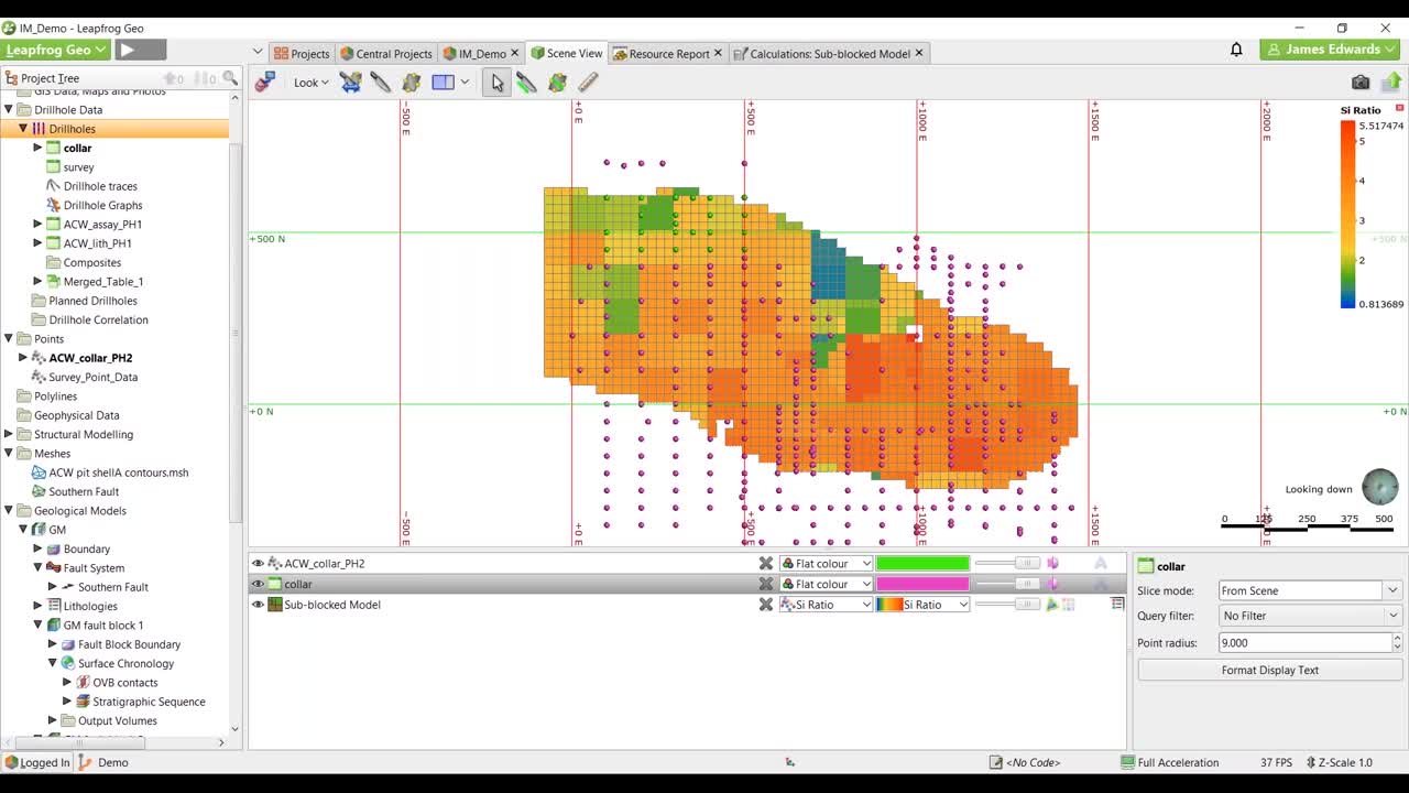
[00:42:46.129]And if I go back to my block model now,

[00:42:47.740]I have an option on my dropdown to look

[00:42:50.150]per block of the silica ratios.

[00:43:09.580]So the last thing we’re going to do

[00:43:10.670]as part of this demonstration

[00:43:12.893]is we’re going to have a look at the feature.

[00:43:14.390]One of the key features, again,

[00:43:15.590]that we’ve talked about during the earlier part

[00:43:17.190]of the presentation around the dynamic update capability.

[00:43:20.870]Now, what we have in this particular project is we have,

[00:43:24.960]we have like our drill holes.

[00:43:28.920]Let’s just look in a plan view.

[00:43:32.466]So I have my drill holes here and

[00:43:36.344]you can see that we’ve got a bit of a gap in our model,

[00:43:39.840]up in the north west corner.

[00:43:42.770]So what we’ve done is, they’ve gone out and they’ve drilled

[00:43:46.870]about 15, 20 new holes to fill in that area.

[00:43:53.140]Now, what I want to do with this is

[00:43:54.910]I want to bring that data into my model.

[00:43:57.530]Now in an explicit model, you’d bring that data in.

[00:44:00.860]You bring that data in and you’d have to go and re digitize

[00:44:05.310]all your strings, go and recreate all your wireframes,

[00:44:09.380]rebuild your models, rebuild your block models.

[00:44:12.840]And that process would essentially take

[00:44:14.610]almost as long as the original model did.

[00:44:18.120]Now, mentally, this model has been pretty quick,

[00:44:20.170]but what we’re going to see is if I go into my drill holes,

[00:44:22.880]I’m going to go and find that second phase of drilling.

[00:44:24.900]So I’m going to go pen that to my current database.

[00:44:29.750]I got to search for my data.

[00:44:30.930]So this case I’ve got my color phase to drill in here.

[00:44:35.860]I’ll open this one up.

[00:44:39.080]So one of the things Geo does is, it searches by name,

[00:44:42.770]So if it finds anything with a similar name, it’ll go,

[00:44:45.170]and pre-populate your survey and read full tables.

[00:44:47.620]You don’t have to go and change that,

[00:44:48.800]but it’s just a nice feature to, again,

[00:44:51.640]hopefully get you moving a bit quicker.

[00:44:53.730]So if I import that data,

[00:44:55.060]it runs through my drill hole and Porter.

[00:44:57.580]These have already been pre set up by the initial import

[00:45:00.600]of the data when I first set the model up.

[00:45:03.300]So I can run through these

[00:45:05.090]because I know they’re all the same.

[00:45:07.644]And what it’s going to do now is it’s going to basically

[00:45:09.290]rerun everything.

[00:45:10.130]So,

[00:45:12.923]the way Geo works is that kind of at the top of your tree

[00:45:15.860]is your drill hole data.

[00:45:16.760]So that is your key,

[00:45:18.650]your cornerstone piece of information.

[00:45:21.140]Everything else you do in this example here

[00:45:24.160]is built off that drill hole data.

[00:45:26.850]So if you add new data to your drill holes

[00:45:30.580]is going to flow through and rebuild your model

[00:45:32.920]based on the rules and parameters you defined

[00:45:35.312]is then going to go and rebuild your block model,

[00:45:37.730]rerun your estimation parameters and,

[00:45:41.150]essentially all the way through to the resource report.

[00:45:43.730]So you can see here in the case of the silica ratio

[00:45:46.080]had in that new drilling has dropped my silica ratio

[00:45:50.000]in this area.

[00:45:51.960]We’re going to have a look at the resource report,

[00:45:53.800]You can see my tonnage has gone up.

[00:45:56.270]And I think by my grades dropped slightly.

[00:46:01.220]But in the, basically in the time,

[00:46:02.580]it took me to explain what I was actually trying to do.

[00:46:05.280]I’ve managed to rebuild the whole model,

[00:46:07.600]re estimate and re report.

[00:46:10.630]Now what we kind of mentioned earlier,

[00:46:12.680]obviously that doesn’t take away from the fact that

[00:46:14.520]if you’re doing this in the real world,

[00:46:16.630]bringing any new data into a project

[00:46:18.290]still requires the initial validation and post validation.

[00:46:21.850]So once all of that’s pre-run,

[00:46:24.170]it’s imperative that the geologists goes back and has a look

[00:46:27.990]in 3D how the impact of that data to make sure

[00:46:30.540]that it’s still true to what you believe should happen

[00:46:34.660]or still make some geological sense.

[00:46:39.700]So essentially the last thing we would normally do

[00:46:41.610]with this is we’ve made a significant change.

[00:46:43.330]We’ve added some new data in, so if we had done this,

[00:46:45.510]we’d go down and we’d publish this model back up to Central.

[00:46:49.530]And that publishing process is pretty straightforward

[00:46:51.830]and nice and quick.

[00:46:52.890]In here you can pick the objects you want to be available

[00:46:55.200]for other people to view.

[00:46:57.010]So in this case, we might just say, well, look,

[00:46:59.620]I’ve made a change to my block model and my geological model

[00:47:02.050]by bringing in my new lithology and assay table.

[00:47:07.210]I’ll leave this stuff for now, like I say,

[00:47:09.300]more than happy to go through more detail with you

[00:47:13.160]in person, anytime after this, I needed to comment onto why,

[00:47:18.210]you’re loading this or

[00:47:19.230]why you’re publishing this new version up.

[00:47:20.910]So in this case, we have some additional drilling.

[00:47:33.086]I want you to, on that, you can click next.

[00:47:35.170]It’s going to run through a process of basically

[00:47:37.470]collecting the data.

[00:47:38.303]It has a look at what’s already in Central.

[00:47:41.470]So what was the previous version?

[00:47:43.300]And it looks at what’s changed in your current model.

[00:47:45.650]So anything that’s changed it based in our packages up

[00:47:48.960]posts up to the Central server

[00:47:51.660]and is now available as a new node on that tree

[00:47:54.430]for essentially anyone to go and have a look at.

[00:47:57.780]Now, if that, if you wanted to be able to just

[00:48:02.910]show somebody the model or provide it to them to look at,

[00:48:06.980]so it could be again, management, external stakeholders,

[00:48:10.060]it might be, you just want to take it out

[00:48:11.500]with you on your phone or an iPad into the pit.

[00:48:13.830]You can also publish the view.

[00:48:16.670]So in 3D with the,

[00:48:17.787]the functionality of spinning it around and turning things

[00:48:20.010]on and off in our View application.

[00:48:23.240]So View application is completely free and it’s web based.

[00:48:27.040]So there’s an option up in the top corner here

[00:48:30.890]where you can choose to publish a view.

[00:48:34.870]And if you upload that it basically runs and provides you

[00:48:37.990]with a web link and that web link can then be provided

[00:48:40.990]to any other user or any other person.

[00:48:44.310]It doesn’t have to be a user of Geo.

[00:48:45.980]They don’t need any particular software.

[00:48:48.570]They just need to be able to use a web link

[00:48:51.910]and have an active connection.

[00:48:57.531]So you can see here in this case,

[00:49:00.350]I can get their address and I could send that address on,

[00:49:07.450]okay, so that’s pretty much all the,

[00:49:09.720]the initial features I wanted to show you, like I said,

[00:49:11.300]it was a very high level, quite quick run through,

[00:49:14.210]but just to see some of the capability of the program

[00:49:16.800]and kind of hopefully visualize some of the features

[00:49:20.403]that I was talking about in the earlier part

[00:49:21.740]of the presentation.

[00:49:24.460]I think the main takeaways you get from this is obviously

[00:49:26.580]the ease of use the speed that you can model and update,

[00:49:32.170]and the dynamic capability of adding new data

[00:49:35.200]into your model.

[00:49:42.300]So we jump back into our presentation

[00:49:44.380]and basically that’s pretty much it from me.

[00:49:47.640]So I want to initially thank you for your time

[00:49:49.540]and I hope you’re able to get some value from the

[00:49:50.980]information presented, but like I said,

[00:49:52.920]the webinar is only an introduction and I personally would

[00:49:55.900]be more than happy to catch up with you.

[00:49:57.010]After the event to discuss how Seequent products

[00:49:58.940]can help your projects

[00:50:00.080]or run through maybe workflow options.

[00:50:02.890]We offer free trials to the software and we run a number of

[00:50:05.380]trainers sessions around the globe,

[00:50:06.580]which are all listed on our homepage.

[00:50:09.100]So lastly, thanks again for joining me

[00:50:10.650]and I hope you have a great rest of the day.