Getting Started In Leapfrog Edge

This webinar we will cover:
• Considerations for the input data
• Setting up the estimators
• How to validate the estimate
• Post processing of the block model and reporting the resources

 

Overview

Video Transcript

[00:00:00.330]<v Instructor>How do I validate my estimate?</v>

[00:00:01.790]Where can I check my top capping stats?

[00:00:04.210]How do I know the search ellipses are orientated correctly?

[00:00:07.910]How do I make a resource table?

[00:00:10.220]These are all common questions we hear

[00:00:11.970]when people are starting out

[00:00:13.130]with Edge or haven’t used it in awhile.

[00:00:15.370]And maybe these will be the kinds of questions

[00:00:17.190]you will be asking yourself if you’re new to Edge.

[00:00:20.070]Hi, I’m Carrie Nicholls,

[00:00:21.380]a senior resource geologist here at Seequent.

[00:00:23.620]And over the next 30 minutes,

[00:00:24.890]I’m going to give you an introduction to Edge

[00:00:27.000]to help you get through that first estimation run.

[00:00:32.370]To start with,

[00:00:33.203]we’ll go through the setup and basic workflow,

[00:00:35.500]which essentially explains how Edge works.

[00:00:38.210]Then we will go through the various visualization tools

[00:00:40.670]available to us to better understand

[00:00:42.640]the statistics and geo statistics,

[00:00:44.720]and also the visual ways to validate your data model.

[00:00:48.480]Finally, we will demystify some calculation syntaxes

[00:00:51.040]in the post-processing

[00:00:53.210]and how to create a simple resource report.

[00:00:56.152]Let’s go into the software.

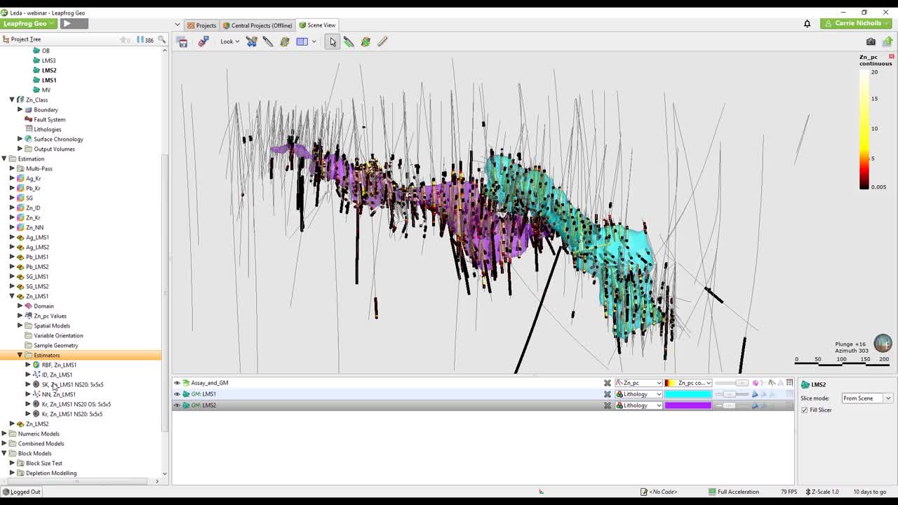
[00:00:57.940]How does Edge work?

[00:00:59.350]When you have the Edge module activated in geo,

[00:01:02.050]you will notice that you have an extra folder

[00:01:03.890]in your project tree called estimation.

[00:01:06.620]This folder will hold all the estimation parameters

[00:01:08.870]that we’ll use as well as defining the inputs,

[00:01:10.900]such as the domain and data.

[00:01:12.640]Also the query filters,

[00:01:13.890]compositing rules, search parameters,

[00:01:16.210]estimation methods, et cetera.

[00:01:17.900]They will be stored in the domain estimators individually,

[00:01:21.580]and then combined into the combined estimator.

[00:01:24.780]The domains then with the associated inputs and parameters

[00:01:28.270]will be evaluated onto the block model.

[00:01:30.090]So this is the second part of the project G

[00:01:32.640]that you’ll be working in.

[00:01:34.560]So in the block model,

[00:01:36.260]you can also do the validation and reporting,

[00:01:39.520]and the results of those

[00:01:40.900]will also be stored on the block model itself.

[00:01:43.710]This means that the outputs that get generated

[00:01:46.530]will be updated if you change any of the inputs

[00:01:48.810]or parameters from the estimation folder

[00:01:50.700]or the underlying meshes in sample data.

[00:01:53.390]This allows you to work efficiently

[00:01:54.840]without having to stop

[00:01:55.870]and reload or rerun processes individually.

[00:01:59.280]However, I would recommend that you make use

[00:02:01.060]of the freeze function on the block models

[00:02:03.620]if you do have a few models linked to the same parameters,

[00:02:06.710]so they don’t all start running at once

[00:02:08.830]with every iteration.

[00:02:11.600]If I come back up to the estimation folder,

[00:02:14.520]you’ll see that there’s two different icons,

[00:02:17.220]the lower ones are the individual domains

[00:02:19.370]for the various variables to be estimated.

[00:02:22.090]In this project, there are two domains,

[00:02:23.850]as you can see in the scene

[00:02:25.740]denoted by these two volumes here.

[00:02:29.729]And the domain estimation has been set up

[00:02:31.970]for each variable and each domain.

[00:02:34.077]And this is how Edge works.

[00:02:36.020]You set up the estimators on a domain by domain basis

[00:02:38.930]for each variable.

[00:02:40.170]So if it’s a polymetallic deposit like this one,

[00:02:43.133]I have to repeat the domain decimeter for each variable

[00:02:45.860]and each domain.

[00:02:47.760]To speed the process up a bit, you can copy the domains.

[00:02:51.260]I’ll just go to one of these now.

[00:02:53.630]When I open it up,

[00:02:55.170]you will see that underneath I have domain and values.

[00:02:58.500]So these are the two input items that define

[00:03:02.000]what this estimation domain is all about.

[00:03:05.460]So again, I’ll drill down and you will see that.

[00:03:08.490]Here are the underlying data for both of these.

[00:03:15.300]So these are defined when you first create your estimator

[00:03:18.360]under the domain here.

[00:03:21.430]Now you can pick any valid volume in your project.

[00:03:24.570]So it doesn’t work with surfaces.

[00:03:26.220]You have to have a volume.

[00:03:29.008]What I mean by about volume

[00:03:30.600]is that it has to be closed and validated.

[00:03:33.250]So if you do not see the volume that you want to use

[00:03:36.060]as your domain in the list, when you come to select it,

[00:03:38.900]it means it’s not valid in leapfrog.

[00:03:42.010]So what I mean,

[00:03:44.990]So I’ll come into the geo model here, for example,

[00:03:49.240]pick an output volume.

[00:03:51.581]If you go to the properties on the mesh

[00:03:53.110]that you want to check, is this part here

[00:03:56.620]you want to have a look at.

[00:03:57.720]The closed, consistent and manifolds that they’re all true.

[00:04:00.860]If any of these are false,

[00:04:01.890]it won’t be a valid volume to be used.

[00:04:06.350]The values are selected here,

[00:04:09.180]and then you can pick that off your drill hole

[00:04:10.990]or your points data.

[00:04:13.020]And then if you want to use a query filter,

[00:04:14.980]then you must also apply a chair.

[00:04:16.460]So this is really important.

[00:04:17.810]If you want to exclude certain data from your data set

[00:04:20.210]because of unreliable data.

[00:04:25.400]You can also set up your compositing rules in here.

[00:04:28.450]The advantage of doing it this stage

[00:04:30.040]within the domain estimation part

[00:04:33.100]is that you can select within boundary

[00:04:36.150]and you’ve got your usual compositing rules

[00:04:38.970]and what to do with the residuals.

[00:04:41.770]And then this chart on the right hand side is a useful chart

[00:04:45.120]for showing you how the grade changes

[00:04:48.310]across the domain boundary.

[00:04:50.720]So the grade is averaged over slices,

[00:04:56.060]gradually inside and outside of the domain.

[00:04:59.520]And you can see here that their grade outside of the domain

[00:05:03.060]is very low and then immediately inside is very high.

[00:05:06.820]So this would be a hard boundary.

[00:05:09.370]And if the grade was much more gradual across the boundary,

[00:05:13.440]I may consider using a soft boundary,

[00:05:15.900]which means that I would include some samples

[00:05:18.100]outside of the domain to be used in the estimation.

[00:05:22.560]You can also use this to validate your domaining.

[00:05:25.890]If you’re expecting a very sharp sample grade

[00:05:29.470]from inside to outside,

[00:05:31.880]and you see that the grade is very gradual,

[00:05:34.550]then you should go back and check your domaining.

[00:05:45.040]So everything else you see underneath the domain

[00:05:51.230]are then the parameters to be used.

[00:05:55.160]You can see that there are four folders

[00:05:56.870]underneath the domain.

[00:05:58.880]We have the spatial models, which is the variography,

[00:06:02.780]the variable orientation.

[00:06:04.080]So that’s, if you want to locally orientate

[00:06:06.840]your search ellipse and your variogram model

[00:06:09.330]during the estimation process.

[00:06:11.220]Sample geometry, if you want to check the D clustering.

[00:06:14.800]And the estimators folder

[00:06:16.130]holds all the estimators themselves.

[00:06:18.340]So you’re not restricted

[00:06:19.370]to just having one estimate in there.

[00:06:21.750]So this is useful if you want to do multi passes,

[00:06:24.410]you can put your multi passes under this folder

[00:06:27.100]for the same domain, with the same samples.

[00:06:29.420]If you want to check different estimation methods,

[00:06:33.140]if you want to try different parameters,

[00:06:35.280]you can put them all into here

[00:06:36.490]because you have to evaluate them onto the block model.

[00:06:40.380]And you don’t have to evaluate everything into the folder,

[00:06:43.440]just the ones that you need.

[00:06:46.300]So the methods available to us are the inverse distance,

[00:06:49.710]nearest neighbor, kriging.

[00:06:51.100]So that’s ordinary kriging and simple kriging and the RBF.

[00:06:59.210]So once you’ve set up all your estimators,

[00:07:02.050]or sorry, and your domains individually,

[00:07:04.600]you will then want to combine them.

[00:07:07.060]So this is just so that on your block model,

[00:07:09.600]you will just have one field that represents

[00:07:12.235]the estimation for let’s just say lead or zinc

[00:07:16.410]in one field with all your multipasses and all your domains.

[00:07:20.800]So when you do create this,

[00:07:22.370]it is important to get the hierarchy correct,

[00:07:25.240]especially if using the multipass.

[00:07:26.730]So I’ll go into my multipass example here.

[00:07:34.680]And you can see, I’ve got multipasses for LMS1 and LMS2,

[00:07:40.070]that’s my two domains.

[00:07:41.640]And then I’ve got Pass1, P1 and P2 here.

[00:07:45.780]So they do have to be in the right order.

[00:07:48.870]So priority towards the top.

[00:07:50.730]So I want my Pass1 to have priority over Pass2.

[00:07:54.110]So when you do this, just double check

[00:07:56.360]that you do have them and in the correct order.

[00:08:00.700]So you can evaluate both the combined and the individual

[00:08:06.170]estimation domains onto your model.

[00:08:08.480]And doing both is useful,

[00:08:10.550]because if you want to validate your parameters,

[00:08:14.500]I would advise you first start off

[00:08:16.080]with the individual estimators

[00:08:18.910]before you move on to the combined ones for the validation.

[00:08:22.940]So when you have set up at least say one domain,

[00:08:26.280]you can come down onto your block model.

[00:08:29.320]So you can create a regular block model

[00:08:32.790]or a sub block model.

[00:08:34.580]And here I have two block models.

[00:08:37.700]One is called validation, one’s called final.

[00:08:40.070]I’ll just expand these out so you can see

[00:08:42.080]what the difference is between the two.

[00:08:44.730]So my validation model,

[00:08:46.180]I’ve put on all the individual estimators,

[00:08:48.730]because at this stage I’m just testing parameters.

[00:08:51.770]I want to test, do check estimates as well.

[00:08:56.430]And then for my final block model,

[00:08:58.490]I’ve really trimmed it down.

[00:08:59.620]I don’t have the individual estimators on there.

[00:09:02.550]I’ve just put the combined estimator

[00:09:05.480]and excluded any unnecessary information.

[00:09:13.610]So I’ll just open the validation one.

[00:09:19.410]So for the block model setup,

[00:09:21.240]you just need to input your grid in,

[00:09:23.970]your extents and your parent block size,

[00:09:26.200]and then your sub block counts.

[00:09:28.470]If you’ve created a sub block model,

[00:09:30.290]you sub blocking triggers.

[00:09:31.510]So that’s just any meshes that you wanted

[00:09:34.010]to sub sale against or sub block against,

[00:09:36.670]the final tab is the evaluation.

[00:09:38.440]So this is what you want evaluated onto the block model

[00:09:41.340]or coded onto the block model.

[00:09:44.000]So that can be any of your geological models.

[00:09:46.630]For example, you might not just have your domain model.

[00:09:49.050]It might be a weathering model, alteration model,

[00:09:52.600]also design models, pick models, depletion models,

[00:09:56.420]that kind of thing that you’ve built up.

[00:09:59.140]And then the estimators themselves.

[00:10:01.160]So this is very easy to put on and off your model.

[00:10:06.540]You can either use the hours or double click,

[00:10:08.340]and it’ll move them to the left or to the right.

[00:10:11.690]And this is just a list of all the estimators on here.

[00:10:23.074]And this next part of the webinar,

[00:10:24.290]I’ll show you the visualization tools

[00:10:26.010]we have to help you with your stats analysis,

[00:10:28.380]the geo stats and your block model validation.

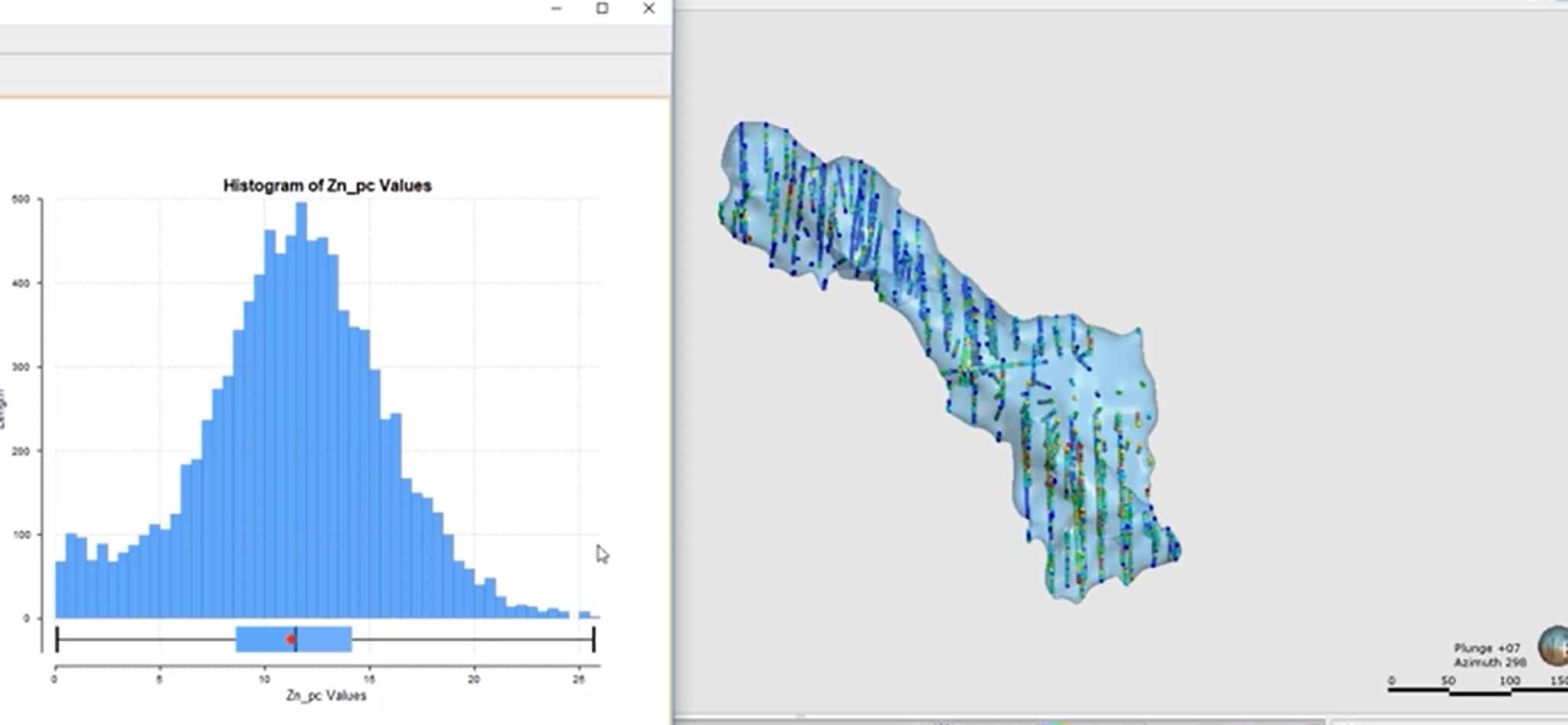
[00:10:32.477]First I’ll show you the histogram.

[00:10:34.460]So I’m coming up to one of my estimators.

[00:10:39.717]I’ll just drag these into the scene.

[00:10:43.390]And I’m just going to do the statistics,

[00:10:46.040]select univariate graphs.

[00:10:49.390]Let me see this histogram here.

[00:10:50.690]Now, this is interactive,

[00:10:52.350]which means that when I select these bins,

[00:10:54.610]it’ll filter out the other sample.

[00:10:56.400]So if I select say these samples,

[00:10:59.170]sorry, these bins at the top here,

[00:11:01.990]you can see that in the scene, it has filtered out

[00:11:03.890]all the other samples.

[00:11:05.565]So this is really useful

[00:11:07.360]when you’re doing a top cap analysis.

[00:11:09.510]If I want to see the spatial distribution of my high grades,

[00:11:12.660]I can easily just come to my histogram

[00:11:15.010]and select some of those bins

[00:11:16.800]to check where they sit in my domain.

[00:11:19.710]Now you see here, the query filter is made on the fly.

[00:11:23.170]You can’t actually save this,

[00:11:24.710]but I can switch it off like this, or back on

[00:11:27.450]or just by deselecting those ins.

[00:11:34.280]So let’s just say,

[00:11:35.140]I’m going to select say a 20 grand button,

[00:11:39.620]sorry, not grand button.

[00:11:40.970]Let’s say percent,

[00:11:42.640]value from a top cap.

[00:11:45.390]I could come down and apply that to one of my estimators.

[00:11:49.979]So I’m just opening the estimator here.

[00:11:56.540]And I will use the top cap of 20 here.

[00:12:10.830]And you can see now it’s made another item

[00:12:13.490]under my estimator,

[00:12:15.090]and this is the, it says clipped values.

[00:12:19.080]So I can also do the stats on this.

[00:12:21.460]And again, I’ve got a histogram.

[00:12:23.650]And again, I can check in the scene.

[00:12:26.660]So now I have to pull these values into the scene,

[00:12:30.490]switch the other ones off.

[00:12:33.120]Let me select that.

[00:12:35.070]And I can see those samples from that bin.

[00:12:38.980]So I can also see the number of samples that I’ve capped.

[00:12:41.870]And I can also check them again in the scene here.

[00:12:44.417]And then these are the statistics associated

[00:12:47.460]with these clipped values.

[00:12:49.670]Clipped and capped mean the same thing in Geo.

[00:12:52.240]Also clumping,

[00:12:54.720]this means, all means the same thing.

[00:12:56.260]It’s all capped to the value that you set it to.

[00:13:07.070]Next, I’ll take you through the visualization tools

[00:13:10.810]to help you with your variogram modeling.

[00:13:13.300]So I’ll come to the spatial models folder.

[00:13:15.140]So that’s where the variograms are stored and made.

[00:13:18.880]And I will just create a new one.

[00:13:24.800]So you can see as I’ve created it,

[00:13:27.250]it’s created this flatter lips.

[00:13:29.440]I’m just going to pull the data into the scene

[00:13:31.380]so we can get some context.

[00:13:38.170]So this is my domain and the samples.

[00:13:40.220]And I can see that my variogram model is flat.

[00:13:43.420]Now, one thing to note here is that

[00:13:45.030]Leapfrog Geo doesn’t do any automatic modeling

[00:13:48.160]of the variogram.

[00:13:48.993]This is an arbitrary model

[00:13:51.206]or values put in and you must model it yourself.

[00:13:56.740]So the principle that it works on is that,

[00:13:59.850]you need to align your variogram

[00:14:02.550]into the plane of your minorization.

[00:14:05.830]So there’s that sense of the major plane

[00:14:07.650]of the minorization.

[00:14:08.880]And then you’ll be confident that each of these,

[00:14:12.903]for your experimental variograms

[00:14:15.070]are in the right directions compared to the major.

[00:14:19.370]because it’s creating the experimental variograms

[00:14:23.260]also going all to the major direction.

[00:14:28.950]So the direction is here.

[00:14:32.570]And the easiest way to do it

[00:14:33.990]is look at the data in your scene,

[00:14:36.220]create a plane, and then use the set from plane.

[00:14:39.410]Of course, you can also just put in your dip estimates

[00:14:41.880]in your pitch if you know it.

[00:14:44.770]So all I’m going to do here

[00:14:46.930]is I’m going to align the scene

[00:14:48.400]so I’m looking down into the plunge of the data,

[00:14:58.560]draw a plane.

[00:14:59.980]So I’m in the plane of the major direction,

[00:15:06.107]and it’s plunging off this way.

[00:15:08.470]Then this way, rather.

[00:15:10.430]I can do set from plane.

[00:15:16.137]I can also switch these off?

[00:15:17.960]And I can see now that my variogram is now

[00:15:22.410]aligned into the plane of the minorization.

[00:15:25.790]So now I’m competent that these variogram

[00:15:27.950]are now all correctly aligned.

[00:15:32.180]And then I can model each one of these individually

[00:15:35.500]in the seat in each individual one,

[00:15:37.160]or I can do it from here.

[00:15:39.339]You can type in the values up here

[00:15:41.480]or just model it on the,

[00:15:46.600]in the scene like this on the graph, sorry, on the chart.

[00:15:49.580]And you can see as I’m doing this,

[00:15:52.800]that the variogram model is actually live updating.

[00:15:57.210]So I just switch off the domain.

[00:16:00.764]I can see that my,

[00:16:04.290]my ellipsis is changing shape to match

[00:16:06.970]the values that I’m putting in.

[00:16:08.150]So you can really check that it makes sense

[00:16:11.260]in terms of your data,

[00:16:12.564]and it’s just the data distribution,

[00:16:14.860]and that is perfectly aligned the way it should be.

[00:16:21.235]I’ve done the left side’s with all

[00:16:22.880]the experimental variogram controls are.

[00:16:26.460]I’m not going to do anything with those.

[00:16:29.580]But I just wanted to show you how best to sets up

[00:16:35.240]the variogram model in the first place.

[00:16:39.990]So I can come out from here.

[00:16:43.260]The ellipse is also available for the search ellipse.

[00:16:46.420]So if you open up one of your estimators

[00:16:49.620]for the inverse distance or the kriging,

[00:16:53.840]you will see that the search ellipse

[00:16:57.470]also comes into the scene.

[00:16:59.130]And this also, if you change these ranges,

[00:17:02.230]they will live updates as well.

[00:17:04.630]So again, you can check that it’s making sense on your data

[00:17:08.470]and it’s aligned correctly.

[00:17:11.260]Cancel that.

[00:17:18.240]Next, I want to show you the block interrogator.

[00:17:24.240]So this is a really handy too

[00:17:26.620]for your block model validation.

[00:17:28.810]So I’m just going to bring in this block model into the scene.

[00:17:37.370]Okay.

[00:17:40.769]And what they block interrogator

[00:17:43.770]or interrogator estimator to work,

[00:17:45.900]you have to have the individual,

[00:17:48.170]or have an individual estimator on your block model.

[00:17:51.680]It won’t work with a combined estimator.

[00:17:54.380]So that’s why I’m using my validate model here.

[00:17:58.270]And what the interrogator does,

[00:18:01.070]is it will display the search volume use

[00:18:03.770]for that block estimate and also the sample selected.

[00:18:07.060]So this is really good for any areas on your block model,

[00:18:10.720]where you want to check if you have extremely high

[00:18:13.450]or extremely low, or say on the peripheries

[00:18:15.490]where you’re not really sure,

[00:18:18.171]or you want to double check while you’re getting

[00:18:20.940]the values that you are.

[00:18:23.310]So for example,

[00:18:24.143]I’ll come up to this top part here

[00:18:25.800]where I’ve got a low value,

[00:18:29.620]select to block.

[00:18:31.805]It just takes a while to load up.

[00:18:35.070]There we go.

[00:18:36.080]Interrogate estimator.

[00:18:39.920]And you can see I’ve got now the search volume

[00:18:42.470]that was used for that block.

[00:18:44.600]Now, this is also really good to validate

[00:18:46.580]your variable orientation,

[00:18:49.270]because then you will be able to check

[00:18:50.950]the locally orientated search ellipse

[00:18:54.240]for blocks in different parts of your deposit.

[00:18:59.960]I’m just going to change some of the parameters here.

[00:19:01.880]So I’m going to change from frame to include it.

[00:19:03.933]That’s what was included in my estimate,

[00:19:06.250]built to the block model.

[00:19:08.170]And now I can just see the samples and the block

[00:19:10.920]that I’m interrogating.

[00:19:12.350]And I’ve got a list of the samples that we used

[00:19:15.380]for the estimate,

[00:19:16.213]and they will correspond to those points in there.

[00:19:19.040]So I can just switch off that search volume.

[00:19:22.940]It’s quite large.

[00:19:25.310]And then if I want to change,

[00:19:26.980]sorry, not if I want to change it,

[00:19:28.030]if I want to de-select or I want to see which samples

[00:19:32.110]corresponds on this list,

[00:19:33.630]I can easily sort by any of these columns.

[00:19:37.290]So for example, I can say I’ve got a negative weight

[00:19:40.690]and maybe want to see where those samples are

[00:19:45.570]so I can check where is,

[00:19:47.840]and maybe then make a decision on my parameters that I used.

[00:19:53.177]And I can open the estimator straight from here

[00:19:55.900]and make any changes that I need to,

[00:19:58.460]and then let it rerun.

[00:20:00.590]So that’s a really, really useful tool

[00:20:04.330]for those block validations.

[00:20:10.980]And lastly, I want to go through the status

[00:20:14.430]on the block model.

[00:20:15.263]Now, this is also really important to understand

[00:20:18.270]if you want to use the calculations.

[00:20:23.380]So that’s the post-processing of your block model,

[00:20:26.350]because that’ll help explain some of the syntaxes

[00:20:28.773]that are available to you.

[00:20:31.230]So I’m just going to zoom out a little bit.

[00:20:35.250]And actually what I’m going to do

[00:20:38.160]is I’m going to swap models.

[00:20:45.870]Not running.

[00:20:47.690]It’s okay.

[00:20:48.523]So this ones has the combined estimator on it for zinc,

[00:20:53.470]and it’s currently being viewed by the status.

[00:20:58.040]So you will see that I’ve got two different color blocks

[00:21:02.960]in the scene here.

[00:21:03.860]So I’ve got purple blocks,

[00:21:05.220]which relate to the, without grade blocks.

[00:21:08.350]So these are blocks that didn’t have an estimate

[00:21:11.160]because my search criteria was such that

[00:21:17.690]nothing was fulfilled in terms of the estimate.

[00:21:20.170]And then my white blocks

[00:21:21.580]are blocks that have a grade associated with them.

[00:21:25.100]I’ve switched off the outside because that’s,

[00:21:27.410]they are blocks all outside of the domain.

[00:21:29.870]So if I just, I can illustrate this

[00:21:32.420]if I take a slice through.

[00:21:34.890]Let’s just select the outside,

[00:21:37.760]splice with to make that a bit bigger.

[00:21:42.300]And then just go through to get a nice section.

[00:21:50.080]So here you can see my,

[00:21:52.320]the outline more or less of my domains in the white blocks.

[00:21:56.390]And then I have these unestimated blocks

[00:21:59.100]on the periphery here.

[00:22:04.710]So you can see without grade.

[00:22:06.440]And then these are normal,

[00:22:09.180]which you can’t see here because it has a grade,

[00:22:11.770]and then these are classes outside.

[00:22:14.250]So that’s really useful then for the calculations.

[00:22:19.300]So I’ll just cancel out of this.

[00:22:22.249]I’m just going to clear the screen,

[00:22:23.580]and then I’ll take you into the calculations.

[00:22:26.490]Lastly, in this last part of the webinar,

[00:22:29.110]there are a couple more topics I want to take you through,

[00:22:31.350]which is the post-processing

[00:22:32.790]and setting up a simple resource report.

[00:22:36.400]So I’ll just come into the calculations and filters first.

[00:22:40.450]You can use a calculations for post-processing

[00:22:42.850]on your models, such as adding bulk densities

[00:22:45.400]and dealing with an estimated blocks.

[00:22:47.610]When you come into this section,

[00:22:49.450]you will see on the right hand side here,

[00:22:51.890]on the far right, you’ll see the syntax and functions,

[00:22:55.450]and then just the left of that

[00:22:57.180]is the data on your block model.

[00:22:59.227]And a quick tip here is that the numeric you have

[00:23:02.820]for the numeric data on your model,

[00:23:04.090]you have the minimax displayed.

[00:23:06.310]So this is really handy as an extra validation step,

[00:23:09.360]particularly, if you have negative grades

[00:23:12.500]and you managed to miss that so far

[00:23:14.770]with all your other checks at that point.

[00:23:17.300]Then if I come back to these syntaxes

[00:23:19.390]under the invalid values,

[00:23:21.310]you’ll see the terms relating to those block statuses

[00:23:24.300]that we were just looking at.

[00:23:26.190]So remember the, without grade,

[00:23:27.970]the outside and normal.

[00:23:30.010]So you can use those in your calculations.

[00:23:32.920]And I’ve done that in the example over here.

[00:23:37.730]So if you use a combined estimator

[00:23:40.290]and you want to assign values to unestimated blocks,

[00:23:43.350]you have to do an extra step to let the software know

[00:23:46.400]that the volume you were working in.

[00:23:49.380]In this case, we are coding within the domain model.

[00:23:52.460]I’ve created a variable at the top here,

[00:23:55.000]and I’ve created it as a variable because I don’t want to,

[00:23:57.420]I don’t need this to be written onto the block model.

[00:24:01.284]And the variable just says,

[00:24:02.750]if the GM is equal to the LMS1, or LMS2 domains,

[00:24:08.230]then code it as min or minoralized zone, basically.

[00:24:11.980]Otherwise call it waste.

[00:24:13.390]So we’re not going to use the waste coding,

[00:24:15.200]but I just need to use the,

[00:24:18.650]if the min equals min in my nested if statement.

[00:24:23.150]So down here in the calculation,

[00:24:24.780]this is a numeric calculation.

[00:24:26.410]So that means the output is going to be numeric.

[00:24:29.700]And then my nested if statement,

[00:24:31.150]the first part is just saying the volume,

[00:24:33.710]or basically saying which volume I’m working in.

[00:24:37.170]Now, remember, this is only

[00:24:38.150]if you’re using combined estimators.

[00:24:40.800]And then this part is then dealing with the grades

[00:24:44.360]and what I want to do is missing grades.

[00:24:47.500]So the first top part is just saying,

[00:24:50.040]if the block status is normal

[00:24:52.340]for the combined zinc multipass,

[00:24:55.470]so that’s this estimator here,

[00:24:57.860]then assign it the value from that combined estimator.

[00:25:02.420]The next line, and the next two lines, rather,

[00:25:04.810]they’re both relating to the block statuses

[00:25:07.290]that are without grade.

[00:25:08.820]So this, these are those purple blocks

[00:25:10.560]that didn’t get an estimate.

[00:25:12.560]Again, defining the variable as the combined estimator,

[00:25:17.370]and then using an and statement.

[00:25:19.030]So, and if the GM equals LMS one,

[00:25:22.210]give it a value of 11.

[00:25:23.640]So this was, this value comes from the statistics

[00:25:27.250]I run on the block model.

[00:25:28.150]This was the average grade for this domain.

[00:25:30.710]And then LMS 2 is assigned a value of 10.

[00:25:35.390]Otherwise thinking it will be zero or classified as outside.

[00:25:40.530]Or you can use these otherwise statuses also as checks

[00:25:44.480]to make sure that your coding has worked correctly.

[00:25:49.440]You would also see I’ve got a filter major.

[00:25:51.370]So this simply just is using the pit volumes

[00:25:54.240]that I’ve coded onto my block model.

[00:25:56.320]So we’re pit volumes equals a stage one.

[00:25:59.800]This is a filter that I can then use in the scene

[00:26:02.660]if I want to filter my blocks, but view by another variable,

[00:26:08.660]if I want to use it in my reporting,

[00:26:10.570]which is usually perhaps we’d want to report

[00:26:13.220]within a set volume.

[00:26:14.770]And when I want to export the block model as well,

[00:26:18.250]I can use the filter.

[00:26:21.670]So I’ll just come into my block model

[00:26:25.250]just to check this calculated field.

[00:26:29.870]So this was my combined estimator for zinc.

[00:26:34.180]So my ZN is supposed to be

[00:26:37.390]where I have values for everything.

[00:26:40.950]So I changed the status there.

[00:26:42.253]And you can see I have no purple blocks,

[00:26:45.150]that they’re all classed as normal.

[00:26:48.390]So I can see that my calculation has worked correctly.

[00:26:51.430]And of course an extra validation

[00:26:52.900]would be then to check the values of individual blocks.

[00:26:58.810]Lastly, I’ll show you how to build a simple resource report.

[00:27:02.250]So I’ll do that on this block model here.

[00:27:06.589]Your resource report.

[00:27:10.570]Now, to use the resource report function,

[00:27:13.020]you have to have a category model on,

[00:27:17.223]or you have a category on your block model.

[00:27:20.490]So whether that’s a geological model

[00:27:23.260]or some kind of fit model or something

[00:27:25.270]that you’ve coded onto your model,

[00:27:26.720]or if it’s actually an alphanumeric coded field.

[00:27:30.570]But you need to category.

[00:27:32.100]So I’m going to use my domain as a category

[00:27:36.060]and then my ZN all,

[00:27:37.940]because then I know all my blocks

[00:27:40.040]within those domains will have a value.

[00:27:42.690]You’d always have no unit.

[00:27:44.010]You have to define the unit first.

[00:27:46.010]So I know this is percent.

[00:27:47.950]And then I I’ve got these invalid arrows.

[00:27:51.080]So this is where blocks have blank values

[00:27:55.720]or unestimated blocks.

[00:27:57.780]So we know, or I know that I haven’t done any estimates

[00:28:00.930]in my LMS three and VOOB.

[00:28:04.620]But just so to get rid of those blocks,

[00:28:07.420]if I use a cutoff of zero,

[00:28:10.890]then I’ve excluded those unestimated blocks.

[00:28:14.030]And also use the cutoff at,

[00:28:16.150]it doesn’t have to be zero.

[00:28:17.180]It can be a whatever reporting cutoff.

[00:28:19.060]So let’s say I’m going to report to 5% sync.

[00:28:22.330]Now, I also don’t want

[00:28:23.720]these unestimated blocks in my report,

[00:28:26.540]so I can customize this.

[00:28:28.350]I can switch off these unknowns.

[00:28:30.630]And also maybe I don’t want to report by domain,

[00:28:33.740]but I don’t want to also go and create a new model

[00:28:37.170]to create a category on my model

[00:28:40.370]to recode just for the minoralized zone.

[00:28:43.280]I can just group these together on the fly in the report.

[00:28:47.840]So I can just call this, mean zone,

[00:28:50.920]and then switch off the others.

[00:28:52.740]And these fields are,

[00:28:53.950]sorry, these columns are totally customizable.

[00:28:56.540]You can change the units and the decimal places,

[00:29:02.710]as well as the headings.

[00:29:04.170]And then when you’ve done all of that,

[00:29:05.440]you can just copy the report out

[00:29:07.840]and paste it straight into Excel or in Word,

[00:29:12.960]ready for your report.

[00:29:15.380]And this takes me to the end of the webinar.

[00:29:17.680]I hope this has given you a good understanding

[00:29:19.470]of how Edge works,

[00:29:20.690]how you can validate your model and create reports.

[00:29:23.450]You can see how self-contained the estimation process is

[00:29:26.590]by working in just a couple of folders,

[00:29:28.940]and you’re not having files scattered all over your project.

[00:29:32.660]The strong visualization tools mean that

[00:29:34.550]you won’t have a misaligned variogram model

[00:29:36.420]of search volume again,

[00:29:38.180]which is the kind of situation that brings you out

[00:29:40.290]in a cold sweat when you discover this kind of mistake,

[00:29:43.060]only after you submitted the model.

[00:29:45.720]The quick reporting tools mean that you don’t have

[00:29:47.769]to constantly bring your data out of the software

[00:29:50.530]to build a pure tables in Excel

[00:29:52.850]after every iteration of the model.

[00:29:55.870]Thanks so much for listening.

[00:29:57.400]And I really hope you’ve learned something.

[00:29:59.700]And hopefully I’ll hear from you soon.