Geosoft 9.9 – Discover the latest enhancements to Oasis montaj, Target and VOXI

This webinar is the best place to learn how the new functionality can improve efficiency in your workflows, give you more flexibility and help you make decisions faster.

Webinar highlights include:

• New Multi-Trend Gridding
• Redesigned 2D and 1D Filtering
• New Matched Filtering and Tilt-Depth Calculations
• Updated Gravity Workflows
• VOXI 2.5D Time Domain EM Modelling
• Improved Interoperability and Central Data Room Support
• Core usability and performance improvements

VOXI 2.5D Time Domain EM is under development and not available for purchase.

Overview

Video Transcript

[00:00:04.310]
<v Geoff>Hello, everyone, and welcome to today’s webinar.</v>

[00:00:07.490]
My name is Geoff Plastow,

[00:00:08.840]
and I will be your online host today.

[00:00:11.430]
I’m senior geophysicist here at Seequent,

[00:00:13.620]
and I’m currently based in Vancouver, Canada.

[00:00:16.670]
Today I will be walking you through some of the updates

[00:00:19.040]
we have added to the latest release of Oasis montaj,

[00:00:21.710]
and Target version 9.9.

[00:00:24.770]
Before we get started, I would like to go over a few items

[00:00:27.630]
so you know how to participate in today’s event.

[00:00:30.580]
During the webinar, you will have the opportunity

[00:00:32.630]
to submit text questions, by typing your questions

[00:00:35.200]
into the chat pane of the Goto Webinar control panel.

[00:00:39.000]
You may send your questions at any time

[00:00:40.580]
during the presentation.

[00:00:42.170]
If we’re unable to answer your question during the session,

[00:00:45.080]
we will respond to you via email in the next 24 to 48 hours.

[00:00:53.470]
Today I’m excited to speak to you

[00:00:54.970]
about our November release.

[00:00:57.470]
There’s something for everyone in this release.

[00:01:00.180]
We’re going to start off reviewing

[00:01:01.510]
some of the core usability and performance improvements.

[00:01:04.750]
Then we’re going to move into new ways to share your data

[00:01:07.640]
using Open Mining format and the Central Data Room.

[00:01:11.070]
These new features are available in both Oasis montaj

[00:01:14.070]
and Target version 9.9.

[00:01:17.190]
Following this, we’re going to take a look at a brand new

[00:01:19.940]
multi-trend gridding algorithm available in Oasis montaj.

[00:01:25.200]
Then we are going to take a look at

[00:01:26.530]
the redesigned 1D and 2D filtering inside of Oasis montaj.

[00:01:31.620]
We’ve added some great new functionality

[00:01:33.580]
to our 2D filtering, including match filtering

[00:01:36.520]
and tilt-depth calculation for your potential field data.

[00:01:40.130]
Following this, we’re going to check out

[00:01:41.620]
our updated gravity workflow,

[00:01:43.710]
with some new improvements we’ve added

[00:01:45.100]
for GM-SYS Profile modeling as well.

[00:01:47.950]
And we’re going to wrap up the webinar by taking a quick look

[00:01:50.680]
at VOXI 2.5D Time Domain EM modeling,

[00:01:54.500]
which is now publicly available.

[00:01:56.880]
Now, let’s have some fun, and we’ll jump into Oasis montaj

[00:02:00.390]
and take a look at the latest update.

[00:02:02.640]
As a quick reminder, what I’m showing you is now available

[00:02:05.620]
in both Target and Oasis montaj version 9.9.

[00:02:09.870]
Upon launching the software, you will notice

[00:02:12.500]
that we have made some improvements

[00:02:13.870]
and additional refinements to our user interface.

[00:02:17.300]
We have enhanced the color contrast

[00:02:18.980]
to differentiate between the objects we have selected.

[00:02:22.420]
In the Geosoft database,

[00:02:24.172]
we have also increased the contrast,

[00:02:25.780]
making it easier to distinguish

[00:02:27.330]
adjacent database records or fiducials.

[00:02:31.240]
With this release, we’ve also improved how we can control

[00:02:34.410]
and view the axis information in 3D views.

[00:02:38.650]
Within the 3D view, we can now click Tools and Settings,

[00:02:42.200]
and then Extents.

[00:02:44.260]
By default, 3D views automatically extend

[00:02:47.210]
to the largest object in your view.

[00:02:49.870]
We can now manually set these extents,

[00:02:52.890]
and we can clip all of the data in your 3D view

[00:02:55.420]
all at once, as well.

[00:02:57.600]
Now, we have the option to set our extents

[00:02:59.930]
to whatever we have visible in our 3D view.

[00:03:03.020]
We can do this by clicking Set Visible Groups,

[00:03:06.040]
and this will resize your 3D view.

[00:03:08.840]
You can now control the labeling of the axis in 3D views.

[00:03:13.180]
We can control the number of decimals

[00:03:15.030]
and increment intervals.

[00:03:17.290]
We can click Tools and Settings, then Visualizations,

[00:03:20.350]
to see all of the options.

[00:03:22.320]
We can turn on and off corner points,

[00:03:24.850]
adjust the number of decimals,

[00:03:26.860]
and set the increment intervals in our 3D views.

[00:03:30.990]
Both Target and Oasis montaj have migrated

[00:03:33.930]
from Microsoft Bing Maps to Microsoft Azure Maps.

[00:03:38.060]
And this gives you the ability to easily insert

[00:03:40.640]
satellite, air photo imagery, and roads

[00:03:43.800]
into your project data.

[00:03:46.040]
We’ve also spent time improving how we import,

[00:03:49.310]
export, and find your geoscience data.

[00:03:52.740]
We’ve improved our import dialogues to make the import

[00:03:55.750]
and import template building process simpler.

[00:03:58.650]
We can create a new database right from the import screen.

[00:04:02.070]
Now, we support the import of column array data,

[00:04:05.590]
such as GPR data, or location versus depth resistivity data.

[00:04:10.610]
You can simply select the channel which represents

[00:04:13.170]
depth and geophysical data, in this case resistivity,

[00:04:17.170]
and set it as a column during the import process.

[00:04:22.150]
We now support the bulk export of maps and grids.

[00:04:26.200]
This is a great timesaver when you’ve created

[00:04:28.160]
a number of maps or dozens of sections

[00:04:30.430]
across your project area, and you want to export them

[00:04:32.930]
as GeoTIFF or PDF or a number of graphical formats.

[00:04:37.130]
You can simply click Maps, then Bulk Export Maps.

[00:04:42.810]
Here, you have a number of options,

[00:04:44.770]
including the resolution, export directory,

[00:04:47.610]
and if you want to prefix them

[00:04:48.840]
with the project title, for example.

[00:04:51.050]
Along the same lines, we can now convert multiple grids,

[00:04:54.210]
all at once.

[00:04:55.730]
Here, it’s great if you need to exchange the output format

[00:04:58.670]
or convert to a Geosoft grid format.

[00:05:02.730]
In the Project Explorer, you can now use

[00:05:05.120]
the Open File Location to open a new Windows Explorer

[00:05:09.070]
at the location of that file.

[00:05:11.150]
This is so useful when you’re working

[00:05:12.920]
with complex directory structures, or working with data

[00:05:15.980]
in different directory locations.

[00:05:18.980]
You will also notice geosurfaces are now

[00:05:21.280]
part of the Project Explorer.

[00:05:23.260]
This gives you more visibility and control

[00:05:25.840]
over your mesh and isosurface data.

[00:05:29.610]
Let’s take a look at some of the new and improved ways

[00:05:32.630]
that you can share data with your team.

[00:05:35.640]
This includes improved interoperability

[00:05:38.900]
and Central Data Room support.

[00:05:43.100]
Back into Oasis montaj, now you can simply right click

[00:05:47.140]
on any grid, geosurface, or voxel in the Project Explorer,

[00:05:51.670]
and you will have the option to export to OMF

[00:05:54.450]
or upload to Central.

[00:05:56.680]
As a quick reminder, OMF stands for Open Mining Format,

[00:06:01.300]
and it’s an open source data exchange format

[00:06:04.210]
that gives you the freedom to exchange vector data,

[00:06:06.660]
such as grids and block models,

[00:06:08.410]
between various software packages,

[00:06:10.400]
including the Leapfrog product suite.

[00:06:12.780]
Here, you can right click on grids, voxels, and geosurfaces,

[00:06:15.967]
and it’ll give you the option to export to OMF

[00:06:18.780]
directly from the Project Explorer.

[00:06:21.200]
This includes the bulk export of data in OMF format.

[00:06:25.020]
You can simply select the items

[00:06:26.520]
that you would like to export,

[00:06:28.340]
and you can add descriptions,

[00:06:29.670]
which is embedded into the OMF file.

[00:06:32.300]
You also have the option to reproject your data

[00:06:34.720]
into a uniform coordinate system,

[00:06:36.910]
to avoid coordinate confusion when the file is being shared.

[00:06:41.430]
Seequent Central is a cloud-based data management

[00:06:44.660]
and model management solution.

[00:06:46.880]
This is integrated into Oasis montaj and Target

[00:06:50.050]
and the Leapfrog product suite.

[00:06:52.400]
All of your grids, meshes, and voxels

[00:06:55.320]
can be uploaded to Central for secure storage,

[00:06:58.200]
version control, and for collaboration with your colleagues.

[00:07:02.360]
Inside Oasis montaj and Target,

[00:07:04.760]
in the upper righthand corner,

[00:07:06.620]
you’ll see your Seequent ID and your name,

[00:07:09.430]
and a little green light indicating that you are signed in.

[00:07:13.480]
Next to this, you will see a cloud icon.

[00:07:16.560]
If you have a Seequent server in your organization,

[00:07:19.800]
you will have the option to click on this little cloud

[00:07:23.240]
and select a server to connect to.

[00:07:25.890]
Once you are connected, you’ll see this little green light

[00:07:28.790]
indicating that you are connected.

[00:07:31.490]
When uploading to Central,

[00:07:32.820]
you can see which server you’re connected to,

[00:07:35.350]
and which project you want to upload your data into.

[00:07:38.410]
You have the option of reprojecting your data

[00:07:40.510]
before uploading, and you can simply select the items

[00:07:43.480]
that you wish to share and upload with your colleagues.

[00:07:47.100]
When you’re ready,

[00:07:47.933]
you can click OK to begin the upload process.

[00:07:51.630]
For OMF exports and for Central uploads,

[00:07:54.700]
we now provide you the option to regrid your voxels

[00:07:57.800]
to a uniform cell design.

[00:08:00.500]
If you click Regrid Voxel,

[00:08:02.190]
you can see all of the options available,

[00:08:04.440]
and you have the ability

[00:08:05.380]
to adjust your cell sizes if needed.

[00:08:08.350]
This regridding option improves compatibility

[00:08:11.160]
with other software suites.

[00:08:13.530]
With this new release, we have also greatly improved

[00:08:16.300]
our support for KMZ and KML files,

[00:08:19.730]
which is an increasingly popular way

[00:08:21.520]
for sharing geospatial data.

[00:08:24.020]
With this latest release,

[00:08:24.990]
you can export your Geosoft database lines vector data

[00:08:28.860]
directly into KML format.

[00:08:31.950]
Now, you can import KMZ and KML file points, lines,

[00:08:36.210]
and polygons onto new or existing 2D maps.

[00:08:43.080]
Now, let’s take a look at the brand new multi-trend

[00:08:45.940]
gridding algorithm available in Oasis montaj.

[00:08:49.590]
Some of the challenges we face when visualizing data

[00:08:52.950]
is being able to intelligently interpolate

[00:08:55.350]
across our measured data points,

[00:08:57.930]
and to identify trends in our data.

[00:09:00.900]
With this latest release of Oasis montaj,

[00:09:03.330]
we introduce a new multi-trend gridding algorithm,

[00:09:06.500]
which excels at enhancing trends that already exist

[00:09:09.390]
in your data, resulting in a more realistic

[00:09:12.100]
and geologically plausible result.

[00:09:15.060]
In some sense, the largest filter that you can apply

[00:09:17.920]
to your dataset is defined by the gridding technique

[00:09:21.020]
you use to visualize your data.

[00:09:23.790]
We want to honor the data, while at the same time

[00:09:26.270]
enhance and provide a valuable image.

[00:09:29.220]
The dataset we’re looking at here on the screen

[00:09:32.140]
is from an airborne magnetic survey.

[00:09:34.890]
We have two grids, and on the lefthand side

[00:09:38.040]
we have the total magnetic intensity

[00:09:40.220]
gridded by the new multi-trend gridding technique.

[00:09:43.450]
And on the righthand side we have the same data,

[00:09:46.410]
gridded with the minimum curvature technique.

[00:09:49.220]
With the new multi-trend gridding,

[00:09:51.040]
you can see that this technique better joins

[00:09:53.490]
linear trends that occur in any direction.

[00:09:56.720]
We’re not forced to pick

[00:09:58.130]
a specific trend enhancement direction,

[00:10:01.050]
and the results do not contain boudinage

[00:10:03.640]
or string of pearls artifacts that we sometimes see

[00:10:07.300]
while using other gridding techniques.

[00:10:10.030]
This gridding routine was developed by Tomas Naprstek

[00:10:12.920]
and Richard Smith of Laurentian University.

[00:10:15.710]
So now, let’s take a closer look

[00:10:17.690]
at how we can use multi-trend gridding.

[00:10:20.450]
I’m going to open a database

[00:10:21.710]
which contains our geophysical data,

[00:10:23.920]
and again, this is an airborne magnetic dataset,

[00:10:26.670]
and I can click Grid an Image, Gridding,

[00:10:29.850]
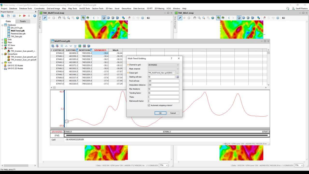
Multi-Trend Gridding.

[00:10:32.120]
Our first step here is to select the database channel

[00:10:34.760]
that we want to grid.

[00:10:35.770]
And we’re going to select our magnetic data.

[00:10:38.910]
I should mention that this gridding technique

[00:10:40.530]
should be used with ground distance units.

[00:10:43.810]
And if your data is using a geographic coordinate,

[00:10:46.610]
such as latitude or longitude,

[00:10:48.950]
it should be reprojected

[00:10:50.290]
into ground coordinates prior to running.

[00:10:52.970]
For example, use UTM zone in meters or feet.

[00:10:57.680]
You will also notice,

[00:10:58.660]
we have an option to set a mask channel.

[00:11:01.640]
I will come back to this in a minute.

[00:11:03.550]
Next, we will select the location and name

[00:11:06.070]
of our output grid,

[00:11:07.550]
and we will have some options for cell sizes.

[00:11:10.800]
By default, the final cell size

[00:11:13.070]
will be two times the size of the starting cell size.

[00:11:17.500]
The starting cell size is used

[00:11:19.240]
for the initial interpolation of the data.

[00:11:22.250]
As a recommendation, the cell size should normally

[00:11:25.140]
be around one-quarter to one-half of the line separation,

[00:11:29.250]
or the nominal data sample interval.

[00:11:32.230]
Once the initial interpolation is complete,

[00:11:34.740]
the gridding method will subsample the entire grid

[00:11:38.060]
to the larger, and sometimes more appropriate,

[00:11:40.390]
final cell size.

[00:11:42.410]
For strong linear features, the small cell size

[00:11:45.140]
can be an asset, making the features smoother

[00:11:47.940]
due to the effect of subsampling.

[00:11:50.040]
With that said, a small cell size must be used with caution,

[00:11:53.950]
as it can remove smaller or weaker lineaments,

[00:11:57.560]
as they now have a further trend, or distance,

[00:12:00.600]
while connecting lineaments.

[00:12:02.410]
Next, we have our interpolation distance,

[00:12:05.030]
and all grid cells within this distance

[00:12:07.630]
are evaluated by the gridding algorithm.

[00:12:10.360]
By default, the interpolation distance is five times

[00:12:13.260]
the starting cell size.

[00:12:15.300]
For our maximum number of iterations, by default,

[00:12:18.660]
this is set to 50 iterations,

[00:12:20.880]
and it defines the number of iterations

[00:12:23.000]
at each grid level refinement.

[00:12:25.600]
Trending factor, the higher the trending factor,

[00:12:28.520]
the smoother the lineaments will be.

[00:12:31.010]
This is typically a number between 0 and 100,

[00:12:33.530]
and by default, it’s set to 50.

[00:12:36.300]
Theta, this is the increment in degrees

[00:12:39.530]
by which to rotate our trend direction.

[00:12:43.040]
By default, this is set to 10 degrees.

[00:12:46.440]
And finally, the multi-smoothing factor.

[00:12:49.300]
The lower the smoothing factor,

[00:12:51.010]
the more unique trending directions are allowed.

[00:12:54.530]
The permissible range is 0 to 100.

[00:12:57.670]
By default, this is set to 0,

[00:12:59.880]
which will find linear features

[00:13:01.310]
in any given azimuth direction.

[00:13:04.640]
Increasing this value will focus on

[00:13:06.650]
predominant linear trends.

[00:13:09.540]
Once we’re happy with our gridding parameters,

[00:13:12.470]
we can click OK to commence gridding.

[00:13:17.770]
Now, we can achieve clearer and more realistic looking

[00:13:20.760]
images of our geophysical data.

[00:13:22.960]
We can join linear features in a realistic way,

[00:13:25.700]
find contacts and trends regardless of their azimuth.

[00:13:31.980]
With this release, the gridding algorithms in Oasis montaj

[00:13:36.020]
can now use a database channel to mask the gridded data.

[00:13:40.680]
This is incredibly useful, and a timesaver,

[00:13:43.420]
if you only need to visualize a part of your dataset,

[00:13:47.350]
or perhaps compare datasets that have different extents.

[00:13:54.070]
Let’s take a quick look at our 1D filtering extension

[00:13:57.100]
for Oasis montaj.

[00:13:59.350]
We have redesigned the filtering to be more visual,

[00:14:02.810]
more intuitive, and more efficient.

[00:14:06.070]
The updated 1D filtering workflow allows you to see

[00:14:09.470]
the effects of the filters in real time,

[00:14:12.380]
while you design them.

[00:14:14.290]
In this example, we’re going to perform a quick filter

[00:14:17.120]
on some noisy magnetic data.

[00:14:19.470]
First, we decide what channel we want to filter.

[00:14:22.840]
Next, we define what the output of our filtered data is.

[00:14:27.230]
Because we’re working with Fourier transforms,

[00:14:29.770]
we need to define the spatial distance increment

[00:14:32.040]
for our data samples.

[00:14:34.040]
Here, you can define this using the average sample spacing.

[00:14:38.510]
Or you can let Oasis montaj calculate this for you.

[00:14:41.750]
Next, we define how our data is interpolated.

[00:14:44.690]
And we can begin designing our filters.

[00:14:47.900]
We can select a filter and define the parameters.

[00:14:51.500]
We immediately see the visual feedback and preview

[00:14:55.010]
of the filtered effect.

[00:14:57.370]
The first filter we are going to apply is a low-pass filter.

[00:15:01.610]
We can test out several filter lengths,

[00:15:03.900]
and immediately see the results.

[00:15:06.470]
This takes a lot of guesswork out of

[00:15:07.900]
the filter design process.

[00:15:10.490]
Again, we can continue to adjust the filter to achieve

[00:15:13.830]
our desired outcome, removing some of the systematic noise

[00:15:17.090]
from our magnetic data.

[00:15:18.800]
In the redesigned 1D filtering,

[00:15:21.150]
the panels that we are presented with

[00:15:22.680]
are resizable and interactive.

[00:15:25.650]
At the top of the screen, we can see the power spectrum,

[00:15:28.670]
and we can move our mouse within the power spectrum

[00:15:31.170]
to more accurately identify wavelengths,

[00:15:33.600]
or wave numbers of interest.

[00:15:36.690]
We can also rescale the spectrum plot, if we’re interested

[00:15:39.670]
in a specific part of the power spectrum.

[00:15:42.010]
With this update, we also see a clear preview

[00:15:45.070]
of the filtered response, the filtered spectrum,

[00:15:48.480]
and the sample profile.

[00:15:50.760]
Once we’re satisfied with the design of our filter,

[00:15:53.520]
we can add another filter if we want,

[00:15:55.820]
and we can see the cumulative effect of both of the filters

[00:15:59.120]
in both the spatial and frequency domain.

[00:16:02.680]
We can switch between the filters.

[00:16:04.460]
We can see the individual and cumulative effects.

[00:16:08.190]
This is incredibly useful, and a real timesaver.

[00:16:11.340]
Once we’re satisfied with the design of our filter,

[00:16:14.060]
we can click OK and Apply,

[00:16:16.850]
and review the filtered results in our database.

[00:16:20.330]
Now you can be more efficient with your time,

[00:16:22.430]
as you design and preview your filtering efforts

[00:16:24.970]
in Oasis montaj.

[00:16:28.640]
Now, let’s take a look at our updated and redesigned

[00:16:31.520]
2D filtering extension, formally known as MAGMAP.

[00:16:36.160]
We made this name change to clarify

[00:16:38.510]
our 2D filtering capabilities extend past magnetic data.

[00:16:43.350]
It can be used on other geophysical data types as well:

[00:16:46.170]
gravity, gravity gradiometry, for example.

[00:16:49.620]
Let’s take a look at the update.

[00:16:51.890]
In this example, I’m using public domain data

[00:16:54.770]
from the Northwest Territories in Canada.

[00:16:58.430]
Using this magnetic grid, we can go ahead and check out

[00:17:01.470]
the new 2D filtering in Oasis montaj.

[00:17:05.000]
We can begin by selecting our input data,

[00:17:07.810]
in this case, our regional magnetic data.

[00:17:11.210]
Next, we need to define our output grid,

[00:17:13.720]
which will be our first vertical derivative.

[00:17:16.630]
Then we need to name our filter file.

[00:17:20.280]
Once we’re ready, we can click Create Filter

[00:17:23.530]
to launch the interactive filtering window.

[00:17:26.390]
Similar to what we saw with the redesigned 1D filtering,

[00:17:30.410]
we can now rescale this window

[00:17:32.710]
along with each one of our panels.

[00:17:35.670]
Inside of the top left panel, we see the power spectrum

[00:17:39.560]
of our input magnetic data.

[00:17:42.130]
In the top right, we see our input magnetic data.

[00:17:46.450]
In the bottom left, we have our filter design panel.

[00:17:50.440]
Let’s go ahead and design our first filter.

[00:17:54.040]
We can click the Filter dropdown list,

[00:17:56.400]
and you’ll see a wide variety of filters and transforms

[00:17:59.380]
that we can apply to our magnetic data.

[00:18:02.730]
The first filter we are going to apply

[00:18:04.710]
is a Butterworth filter.

[00:18:06.570]
This is a commonly used filter

[00:18:08.810]
to suppress unwanted frequencies from potential field data.

[00:18:13.300]
What’s great is now that we have selected

[00:18:15.900]
and started defining our filter,

[00:18:18.040]
we automatically see a preview

[00:18:20.180]
of what the filtered grid looks like.

[00:18:23.170]
We can adjust the filtering parameters, in this case,

[00:18:26.540]
our cutoff wavelength, to resolve longer wavelength

[00:18:30.400]
or deeper structures.

[00:18:33.140]
In our spectrum window, we can see a clear view

[00:18:36.160]
of the original spectrum in black,

[00:18:38.890]
the filtered spectrum in red,

[00:18:41.010]
and the filter response in blue.

[00:18:43.660]
All of this is dynamically updated

[00:18:45.990]
as we update the filter design.

[00:18:48.990]
This is currently a low-pass Butterworth filter,

[00:18:52.660]
and we are stripping away short wavelength,

[00:18:55.670]
or near-surface content, from our magnetic data,

[00:18:59.080]
revealing the long wavelength magnetic structures.

[00:19:03.280]
Now, if we want, we can flip this from low-pass filter

[00:19:07.130]
to a high-pass, passing through the high frequency content,

[00:19:11.550]
or short wavelength data, in our magnetic grid.

[00:19:16.140]
We can see the updated filter spectrum in red,

[00:19:19.280]
and filter response in blue.

[00:19:21.550]
We are now removing the long wavelength content

[00:19:24.570]
from our data.

[00:19:26.060]
We can use the Zoom tool on the righthand side

[00:19:29.420]
to zoom into an area of interest within the input data.

[00:19:33.350]
To further accentuate the near-surface magnetic lineaments,

[00:19:37.200]
we can perform a first vertical derivative.

[00:19:40.190]
This will further suppress longer wavelengths

[00:19:43.080]
and visually sharpen the contacts and dikes we see

[00:19:46.030]
in our magnetic dataset.

[00:19:48.100]
We can see the results of each of the filters independently,

[00:19:52.400]
or how they appear while they’re applied sequentially,

[00:19:55.300]
or stacked.

[00:19:57.720]
Now we can work more efficiently, by fine-tuning our filters

[00:20:00.870]
and transforms and seeing the results instantaneously.

[00:20:05.440]
Once we’re satisfied with our filter design,

[00:20:08.370]
we can go ahead and click OK to apply these.

[00:20:11.950]
This update allows you to fine-tune your filters

[00:20:14.210]
and transforms and get instant visual feedback.

[00:20:17.920]
Now you know if your filter design is heading

[00:20:19.840]
in the right direction in a much more intuitive way.

[00:20:25.000]
Our updated 2D filtering now includes a match filter

[00:20:29.040]
and tilt-depth calculation.

[00:20:31.520]
The match filter is a new feature that will allow you

[00:20:33.980]
to design complementary matched filters

[00:20:36.770]
for interactive depth slicing.

[00:20:39.520]
The tilt-depth calculation is also new, and allows you

[00:20:43.180]
to calculate the tilt-depth to magnetic source,

[00:20:46.030]
to assist with potential field interpretation.

[00:20:50.380]
To launch matched filtering, you can click on 2D Filtering,

[00:20:54.210]
then Matched Filtering.

[00:20:56.280]
Similar to our 2D filtering,

[00:20:58.220]
we have a movable and resizable window.

[00:21:01.030]
The match filters are tapered band-pass filters

[00:21:04.170]
that collectively cover the entire spectrum.

[00:21:07.550]
The first filter is a low-pass.

[00:21:10.000]
The last filter is a high-pass.

[00:21:12.670]
And the in between filters are band-pass filters.

[00:21:16.420]
You may design up to a set of four complementary matched

[00:21:19.620]
filters, to separate the equivalent magnetic response

[00:21:23.090]
at different depth slices.

[00:21:26.190]
Let’s start by selecting our input magnetic grid.

[00:21:29.820]
We have the option of creating a prefix for our grid,

[00:21:32.810]
and we can select the number of equivalent depth slices

[00:21:35.320]
we would like to create.

[00:21:37.460]
For each of the depths, we can enter in a value,

[00:21:40.120]
and you will see the spectrum automatically update

[00:21:42.680]
with the filter designed to extract this slice.

[00:21:46.680]
You may also use the interactive spectrum tool

[00:21:49.330]
to determine an ideal depth slice to extract

[00:21:51.570]
from your data.

[00:21:53.707]
In the spectrum plot, we will see the central wavelength

[00:21:55.830]
for each one of the depth slices.

[00:21:58.690]
And now, in the bottom righthand corner,

[00:22:01.130]
we will see a preview of this depth slice.

[00:22:04.120]
The central wavelength of these filters

[00:22:06.160]
is equivalent to the central depth of these slices.

[00:22:10.140]
And of course, you can preview each of the match filter

[00:22:12.690]
slices before you commit your filter.

[00:22:15.460]
When you are ready, you can click OK

[00:22:17.440]
to extract these depth slices.

[00:22:20.210]
This new match filtering feature was designed for faster,

[00:22:23.670]
more intuitive, and visual interpretation

[00:22:26.050]
of your potential field data.

[00:22:29.270]
We have also included a new tilt-depth calculation

[00:22:32.740]
in our 2D filtering menu.

[00:22:35.780]
You may select 2D Filtering, then Tilt Derivative.

[00:22:39.290]
You will need to select your input magnetic data

[00:22:42.250]
and outputs for both the tilt-angle derivative

[00:22:45.270]
and the output of the total horizontal derivative

[00:22:48.100]
of the tilt-angle derivative grid.

[00:22:50.600]
And finally, the name of the database

[00:22:52.760]
which will contain the tilt-depth calculation.

[00:22:55.770]
This is a simple and fast method to locate

[00:22:58.650]
vertical contacts and determine depth estimates.

[00:23:02.330]
The calculated depths will be stored in a new database

[00:23:05.140]
and can be plotted, gridded, and integrated

[00:23:07.810]
with your interpretation project.

[00:23:10.690]
Because this method uses a first order derivative,

[00:23:13.650]
the method is potentially less sensitive to noisy data,

[00:23:16.520]
compared to methods relying on higher order derivatives.

[00:23:19.720]
And there’s no clusters of solutions to sort.

[00:23:23.100]
From these depth calculations, we can advance

[00:23:25.400]
our understanding of the subsurface

[00:23:27.470]
and integrate these results with other depth source methods

[00:23:30.100]
to confirm our interpretation hypotheses.

[00:23:36.420]
Switching gears a little bit,

[00:23:38.200]
our team has added some new gravity workflows

[00:23:41.060]
in the latest release of Oasis montaj 9.9.

[00:23:44.770]
Let’s take a look at what we have updated.

[00:23:49.450]
In this latest release, you can now correct for

[00:23:52.370]
variable water levels in your gravity terrain corrections.

[00:23:56.850]
This is an important step, if you have multiple lakes

[00:24:00.530]
at variable elevations within your project area.

[00:24:05.500]
We have also improved our support for importing

[00:24:08.820]
Scintrex CG-5 gravity meter data.

[00:24:12.030]
We’ve also implemented the Nettleton method,

[00:24:14.700]
saving you time while automatically looping through

[00:24:17.550]
multiple Bouguer correction densities.

[00:24:20.950]
We’ve also provided a standalone latitude correction,

[00:24:24.470]
which is useful for calculating normal gravity

[00:24:26.730]
for your project.

[00:24:28.470]
We’ve also made updates to our moving platform gravity.

[00:24:31.950]
We’ve added a new time-based low-pass Blackman filter,

[00:24:35.530]
added new gravity leveling tools.

[00:24:38.170]
There’s a QC submenu to identify and process repeat lines.

[00:24:42.200]
You can now easily produce a detailed report

[00:24:44.530]
and visualize repeat or stacked survey lines.

[00:24:48.070]
And we have the ability

[00:24:49.010]
to reconstruct raw gravity from field components.

[00:24:53.470]
Our team has also improved

[00:24:55.370]
the functionality of GM-SYS Profile.

[00:24:58.300]
You can now easily display a georeferenced grid or image,

[00:25:01.900]
through a new workflow,

[00:25:03.260]
allowing the integration of raster data in GM-SYS Profile.

[00:25:07.630]
This means you can now display gridded data

[00:25:09.990]
in plan view or section view,

[00:25:12.380]
and you can display interpretations from Leapfrog,

[00:25:15.220]
seismic, or MT data, georeferenced right inside

[00:25:18.470]
of your GM-SYS project.

[00:25:21.860]
Now, with GM-SYS Profile, we support a new model document.

[00:25:26.050]
The new model document supports easy backups

[00:25:28.630]
and sharing of your models.

[00:25:31.260]
You also reduce the risk of losing data.

[00:25:34.640]
Now, instead of having to manually search and archive

[00:25:37.310]
your project files, you can now simply save the model,

[00:25:40.720]
and all of the relevant project files

[00:25:42.680]
will be archived into a single project file.

[00:25:46.560]
Following our early adopter program

[00:25:48.510]
for VOXI 3.5D Time Domain EM,

[00:25:52.110]
Oasis montaj 9.9 now includes improvements

[00:25:55.610]
to the user experience, algorithm robustness,

[00:25:58.460]
and computational speed in the cloud.

[00:26:01.560]
Forward and inverse modeling in 2.5D is available

[00:26:04.880]
as a beta function to VOXI Time Domain EM subscribers.

[00:26:09.073]
VOXI 2.5D Time Domain EM will be a breakthrough

[00:26:12.430]
for users of time domain data in 3D geological environments,

[00:26:16.890]
including hard rock, salt water intrusions,

[00:26:19.830]
and contamination mapping.

[00:26:21.500]
VOXI is accessible through monthly and annual subscription,

[00:26:24.890]
as well as enterprise agreements

[00:26:26.840]
and pay as you go purchases.

[00:26:29.470]
Geophysicists interested in our existing stage 1D algorithm

[00:26:33.290]
will continue to benefit

[00:26:34.500]
from its numerous and powerful capabilities,

[00:26:36.960]
and will receive access

[00:26:38.490]
to the 2.5D algorithm as a value-add.

[00:26:42.050]
You may visit the online VOXI store at myseequent.com

[00:26:45.930]
if you’re interested in a trial

[00:26:47.330]
of VOXI Time Domain EM modeling.

[00:26:50.600]
Thank you so much for your time today.

[00:26:52.850]
If you would like to find out more about this release,

[00:26:55.550]
please check out the release page at myseequent.com.

[00:26:59.340]
To install the latest update,

[00:27:00.890]
you can simply click Check for Updates in the software,

[00:27:04.580]
or visit myseequent.com.

[00:27:07.530]
Thanks again, and bye for now.