Geophysics for Geologists

Learn about how you can utilize geophysics to add value to your exploration project.

Find out how it is possible to use geophysics to generate more knowledge and value for your geological data, and facilitate decision-making in your exploration project. Some items discussed in the webinar include:

• 2D Filtering of Magnetic and Gravimetric data to aid in interpretation
• Utilizing ternary maps for Gamma-Ray Spectrometry analysis
• Inversion of geophysical data to generate 3D models of physical properties using VOXI
• Integrating geophysical and geological data in 2D and 3D environments to generate meaningful interpretation

Overview

Video Transcript

[00:00:00.429](upbeat music)

[00:00:10.114]<v Kanita>Hello, and welcome to today’s webinar</v>

[00:00:14.220]about Geophysics for Geologists.

[00:00:16.430]I’m Kanita Khaled, a geophysicist here at Seequent,

[00:00:19.360]working from the North American office in Toronto Canada.

[00:00:23.350]During this webinar,

[00:00:24.220]we’ll be taking a look at a variety of topics

[00:00:26.880]in geophysics that are relevant to geologists

[00:00:29.886]in the mining and mineral sector.

[00:00:31.470]We’ll begin with a brief introduction to geophysics.

[00:00:35.040]Then we will go into exploring Pre-Competitive Data

[00:00:38.320]or geoscientific datasets that are open-sourced, free

[00:00:42.150]and ready to use to kickstart your exploration project.

[00:00:46.950]Next, we will explore

[00:00:48.550]some of the most common geophysical methods in mining

[00:00:51.560]and exploration,

[00:00:52.567]including magnetics, gravity, and radiometrics.

[00:00:59.920]Once a geophysics survey is completed,

[00:01:02.200]you will receive several deliverables,

[00:01:04.130]including grids, maps, databases and reports.

[00:01:07.860]We’ll take a brief look

[00:01:08.920]at how some of these key deliverables

[00:01:11.160]can be applied to a mining project.

[00:01:14.186]In the second half of the webinar,

[00:01:16.440]we’ll dig deeper

[00:01:17.278]into how you can get more out of your gridded data products

[00:01:20.660]that you received

[00:01:21.810]and take your data from 2D to 3D

[00:01:25.010]by performing inversions of geophysical data.

[00:01:29.670]Finally, we’ll take a look at a case study

[00:01:32.400]of how integrating your multidisciplinary data

[00:01:35.760]such as geophysics, geochemistry and geology,

[00:01:38.870]in both 2D and 3D environments can really help drive

[00:01:42.230]your exploration and mining activities.

[00:01:52.570]So why geophysics?

[00:01:54.450]Geophysics can be a powerful tool to provide knowledge

[00:01:57.060]and value to a mining or exploration project.

[00:01:59.820]Depending on the type of deposit under review,

[00:02:02.680]a variety of geophysical methods are available

[00:02:05.080]to be used via airborne, ground or borehole applications.

[00:02:11.051]If carefully considered and applied,

[00:02:13.570]the correct geophysical technique can reveal

[00:02:16.050]valuable subsurface information,

[00:02:18.496]reduce overall project expenses

[00:02:20.680]associated with the drilling programs

[00:02:23.340]and also avoid costly mistakes.

[00:02:27.620]Once geophysical data are acquired

[00:02:29.280]over a region of interest,

[00:02:30.680]it holds the potential for even further value.

[00:02:34.600]Understanding the geophysical dataset, its limitations,

[00:02:38.980]its advantages and its interpretability,

[00:02:42.300]is the key to unlocking the value

[00:02:44.000]in a mining exploration project.

[00:02:49.770]Okay, so what is geophysics?

[00:02:52.370]Well, the dictionary definition tells us

[00:02:54.660]that geophysics is the subject

[00:02:56.410]of natural science concerned with the physical processes

[00:03:00.640]and properties of the Earth

[00:03:01.890]and it’s surrounding space environment,

[00:03:04.520]and that we apply quantitative methods

[00:03:07.000]or the analysis of these physical properties.

[00:03:10.700]Today, we’re talking about the mineral exploration group

[00:03:14.300]where geophysics is very widely used

[00:03:17.010]and there’s a variety of methods applied

[00:03:19.700]or some of these goals below.

[00:03:24.070]We’re trying to understand the physical properties

[00:03:26.770]of the subsurface at either a regional or a project scale.

[00:03:31.610]We may be interested in inferring the presence

[00:03:36.220]and position of mineralized bodies

[00:03:38.170]that can be potentially mined or are of economic interest.

[00:03:42.260]We’re interested in inferring the target style

[00:03:44.420]of mineralization or alteration processes.

[00:03:47.920]We may also be interested in mapping structures,

[00:03:50.520]like faults, folds or intrusives.

[00:03:59.068]So when to use geophysics?

[00:04:01.260]Depending on the nature of the target

[00:04:02.980]that we’re trying to map or see,

[00:04:05.300]the geophysical method of choice

[00:04:06.900]needs to be carefully considered.

[00:04:10.620]This chart here displays various geophysical methods,

[00:04:14.400]gravity, magnetic, seismic refraction,

[00:04:17.127]EM, magneto-telluric.

[00:04:20.940]And two columns over here,

[00:04:24.110]we have the associated physical property

[00:04:25.970]that’s being measured by that method.

[00:04:28.130]So during a gravity survey,

[00:04:30.330]you’re measuring density or you’re studying density.

[00:04:33.810]During a magnetic survey, you’re studying susceptibility.

[00:04:37.260]During a Magneto-telluric survey,

[00:04:39.220]you’re studying resistivity.

[00:04:43.490]These are the rock properties

[00:04:45.140]that dictate the geophysical results.

[00:04:48.370]Depending on the nature of the target or ore

[00:04:50.910]and the surrounding host rock,

[00:04:52.130]you’ll want to consider the method

[00:04:54.070]that will display the most contrasting values

[00:04:56.850]in order to map your target.

[00:04:58.920]So if you have knowledge of the rock properties

[00:05:01.790]of the area of interest,

[00:05:03.800]it needs to be considered carefully.

[00:05:07.640]For example,

[00:05:08.690]if it’s known that the mineralization

[00:05:10.590]is controlled by disseminated sulfides which are chargeable,

[00:05:14.470]you may want to conduct an IP survey,

[00:05:17.020]so that you can map conductivity and resistivity.

[00:05:22.040]You can also combine multiple geophysical methods

[00:05:24.960]to gain more knowledge.

[00:05:26.000]Another example, conductive ores can also be magnetic,

[00:05:30.260]so a magnetic survey can be paired with other methods.

[00:05:40.200]Considerations of a geophysical survey.

[00:05:43.900]Before carrying out a survey, a cost study is important.

[00:05:47.520]The cost study of the survey will largely depend

[00:05:49.900]on the method and the size of the area you wish to survey.

[00:05:53.497]This image to the right shows

[00:05:56.116]the survey area that can be mapped

[00:05:58.570]using a geophysical method, normalized by the cost.

[00:06:04.790]For example,

[00:06:05.860]an airborne magnetic or radiometric survey

[00:06:08.380]will cover a lot more ground per dollar

[00:06:11.220]than a helicopter-borne electromagnetic survey.

[00:06:16.280]This is where you’ll also want to consider

[00:06:18.090]the spatial resolution of the survey,

[00:06:20.090]which will be dictated by the size of the target

[00:06:23.020]that’s being mapped.

[00:06:24.840]A small target would require a higher resolution survey.

[00:06:28.520]Talk to your geophysics contractor to work this part out.

[00:06:31.960]Depending on the method used,

[00:06:33.290]keep in mind the survey timeline, weather,

[00:06:37.130]site accessibility and local infrastructure.

[00:06:40.010]All of these will play important roles

[00:06:42.280]in survey design and cost.

[00:06:50.480]Next we’re diving into pre-competitive data.

[00:06:57.210]Depending on the location of the project,

[00:06:59.060]there may already be sources of pre-competitive

[00:07:01.500]or publicly available geoscientific data

[00:07:04.280]that’s ready to use for a cost or at times for free.

[00:07:09.530]These government curated service

[00:07:11.120]can provide the foundation for early stage exploration

[00:07:14.850]and are generally made available by governments

[00:07:17.330]who want to attract mineral exploration investment

[00:07:19.460]into their countries or jurisdictions.

[00:07:23.190]This can be utilized

[00:07:24.860]far before conducting a local scale geophysics survey,

[00:07:28.330]and even far before our drilling program

[00:07:32.090]and further exploration down the line.

[00:07:38.410]So how can you access this data?

[00:07:40.590]Well, government curated geoscience science websites

[00:07:43.940]and data portals will allow you free

[00:07:46.330]or paid access to nation

[00:07:48.410]or region wide geophysical, geochemical, geological

[00:07:52.510]even historical global datasets

[00:07:55.220]and other datasets depending on their mandate.

[00:07:58.350]Some examples include the Tellus program in Ireland by GSI.

[00:08:03.160]GTK, geological survey of Finland.

[00:08:05.570]And in my part of the world,

[00:08:06.990]there was a wealth of information available for Ontario

[00:08:10.510]through the MNDM website.

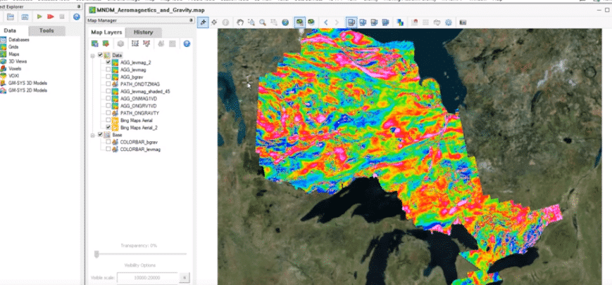
[00:08:17.630]Here is a compiled airborne magnetic grid

[00:08:19.850]over Ontario that I’ve downloaded from the MNDM website

[00:08:23.270]and brought directly into Oasis Montaj.

[00:08:26.210]Within Oasis Montaj,

[00:08:27.500]you easily access publicly available data

[00:08:30.910]by using the Seeker Tool to browse for what’s available

[00:08:34.700]in any given area of interest.

[00:08:39.010]Here, once I go into results,

[00:08:41.100]I can see that over this area of interest,

[00:08:43.770]there is a lot of knowledge

[00:08:45.770]and data that I can download directly into my project.

[00:08:49.400]Data types include gravity, magnetics, geology

[00:08:52.980]and topography.

[00:08:55.760]This data can be easily packaged

[00:08:57.430]and downloaded into your project for further investigation.

[00:09:02.520]Next, we will talk

[00:09:03.550]about common geophysical methods applied to exploration.

[00:09:11.730]We’ll start with magnetics.

[00:09:13.490]Magnetic methods are very commonly used in exploration.

[00:09:17.120]This method is an indirect way to see beneath the Earth

[00:09:19.920]by sensing differences in Earth’s the own magnetic field.

[00:09:23.430]The operative physical property here

[00:09:25.190]has been magnetic susceptibility.

[00:09:27.480]We know that the Earth’s magnetic field strength

[00:09:31.052]can vary greatly from the equator to the poles

[00:09:33.730]and your physicist

[00:09:34.570]can measure this magnetic field intensity

[00:09:37.070]using magnetometers.

[00:09:39.110]These magnetometers can be carried on an aircraft,

[00:09:41.810]by ground or on a boat.

[00:09:44.610]Magnetic surveys are useful

[00:09:45.970]for delineating banded iron formations,

[00:09:48.480]skarn mineralization,

[00:09:49.830]mapping hydrothermal alteration, locating faults

[00:09:53.320]and even defining subtle lithological contacts.

[00:09:58.340]Surveys can be carried out really anytime of the year,

[00:10:00.910]but since the Earth’s magnetic field

[00:10:02.610]can vary with solar activity,

[00:10:04.550]magnetic storms can affect the data

[00:10:07.810]and data acquisition will need to be closely monitored

[00:10:10.240]during the stormy periods.

[00:10:14.820]The deliverables of an airborne magnetic survey

[00:10:17.130]are typically in the format of profile and gridded data.

[00:10:20.570]Routine data processing, and data preparation

[00:10:23.130]of magnetic data includes diurnal variation removal,

[00:10:26.480]correcting for instrument lag or aircraft heading

[00:10:30.650]and also performing tie-line leveling.

[00:10:33.380]Typically when a magnetic map is delivered,

[00:10:35.400]the color ramp or the color legend

[00:10:37.270]is chosen such that the blues are the lowest values

[00:10:40.430]while the reds and the pinks

[00:10:42.940]denote the highest readings of the magnetic field intensity.

[00:10:46.820]In this image,

[00:10:47.990]we have a screen capture of a dataset using Oasis Montaj

[00:10:52.150]where we’re simultaneously visualizing gridded data,

[00:10:55.517]the profile data along which the survey line was carried out

[00:10:59.910]and the associated numerical data.

[00:11:04.570]Let’s go a bit further into some of the key deliverables

[00:11:07.510]you’ll receive with a magnetic survey.

[00:11:10.940]In general, the deeper the magnetic source,

[00:11:13.840]the broader and gentler the gradients

[00:11:16.960]of the resulting anomaly will be.

[00:11:19.170]Also the shallower the magnetic object,

[00:11:21.970]the sharper and narrower that resulting anomaly.

[00:11:25.140]The (inaudible) maps can show anomalies

[00:11:27.290]that have been filtered for size

[00:11:29.210]and shaped to emphasize either shallow or deep sources.

[00:11:33.760]In this image, we have the Total Magnetic Intensity grid.

[00:11:38.810]We see dipoles that are associated with this dataset,

[00:11:45.130]applying reduction to pole

[00:11:46.640]or RTP can simplify this complex dipole effect

[00:11:50.470]and center the anomaly

[00:11:52.020]over the body that is generating that anomaly.

[00:11:55.970]Another derivative method.

[00:11:57.440]The first vertical derivative can magnify magnetic radiance

[00:12:01.410]in the vertical direction.

[00:12:04.300]Where the magnetic field changes from a high

[00:12:07.400]to a low or vice versa.

[00:12:09.710]These derivative grids are often visualized in black

[00:12:13.200]and white and overlain on the total magnetic field map

[00:12:16.730]to really pull out gradients zones,

[00:12:19.110]places that often marked edges of a rock unit,

[00:12:21.820]faults or dyke swarms.

[00:12:24.640]And finally, the image to the right,

[00:12:26.820]we have the Analytics Signal.

[00:12:29.750]The outlines of a geological boundary

[00:12:32.110]can be determined by tracing the maximum amplitudes

[00:12:35.610]of the analytic signal,

[00:12:36.990]which can then help us define the boundaries

[00:12:39.570]of the source causing the anomaly.

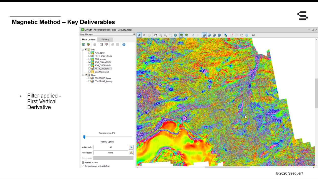
[00:12:44.510]To demonstrate the value of these filters,

[00:12:46.560]let’s look at an example.

[00:12:48.920]This is part of the Total Magnetic Intensity Grid

[00:12:51.340]of Ontario, downloaded MNDM website

[00:12:53.430]and pulled into Oasis Montaj.

[00:12:55.990]Let’s see what it looks like

[00:12:57.060]after applying the first vertical derivative filter.

[00:13:02.220]After applying the first vertical derivative filter.

[00:13:04.510]on this magnetic dataset,

[00:13:06.050]notice how some of the finer structures

[00:13:08.440]are now more prominently visualized.

[00:13:11.150]We can see lineaments that were previously not easily seen

[00:13:13.970]in the Total Magnetic Field Grid.

[00:13:15.810]So the appropriate filter

[00:13:17.910]can significantly improve the interpretability of your data,

[00:13:21.530]but must be applied with caution

[00:13:23.140]and good understanding of the filter.

[00:13:27.400]Next we move on into gravity.

[00:13:30.720]Without gravity, our feet would not be on the ground.

[00:13:33.910]Gravity keeps everything around us in place.

[00:13:36.410]It’s the force of attraction between two bodies,

[00:13:38.670]such as the Earth and ourselves.

[00:13:41.227]The strength of that attraction

[00:13:42.830]depends on mass of the two things

[00:13:45.620]and the distance between them.

[00:13:48.690]A mass falls into the ground with the velocity.

[00:13:50.940]and the rate of increase is called gravitational attraction,

[00:13:54.369]G or gravity.

[00:13:58.040]The image to the right here displays the Bouguer anomaly map

[00:14:01.741]compiled from Ontario’s MNDM dataset.

[00:14:07.780]During a gravity survey,

[00:14:09.040]you’re looking for gravity readings that are high

[00:14:12.360]or low to define your anomalies.

[00:14:14.700]Where you have heavy and dense rocks with a lot of mass,

[00:14:18.120]like from a Chromite, Hematite or Barite in the subsurface.

[00:14:23.140]There is more gravitational attraction

[00:14:25.250]resulting in higher readings.

[00:14:27.268]And where you have rocks with low mass like Halite

[00:14:30.820]or weathered Kimberlites

[00:14:32.350]you’d expect a low reading.

[00:14:35.160]So the operative property

[00:14:36.910]that is being studied here is density.

[00:14:40.460]Gravity surveys are conducted with gravimeters,

[00:14:43.230]and the unit of measurement is milligals.

[00:14:46.760]And the surveys can be airborne, ground or marine.

[00:14:50.590]Gravity surveys are very useful for regional mapping,

[00:14:54.380]identifying structures and at times ore bodies themselves.

[00:15:01.350]When using gravity methods,

[00:15:03.140]the data will need to be processed

[00:15:04.660]and corrected using routine procedures like data reduction.

[00:15:08.260]The goal with data reduction

[00:15:10.550]is to remove known effects caused by predictable features

[00:15:14.410]that are not part of the target.

[00:15:18.070]The remaining anomaly after correction

[00:15:19.870]is then interpreted

[00:15:20.990]in terms of subsurface variation of density.

[00:15:25.920]Each known effect is removed from observed data.

[00:15:30.350]Corrections include latitude corrections,

[00:15:34.300]Free-Air corrections.

[00:15:35.950]Since measurements at higher elevations will be smaller.

[00:15:39.390]We’ll need to correct for that, that’s Free-Air.

[00:15:42.300]Then we have the Bouguer, which further corrects for mass

[00:15:46.440]that may be between sea level and the observer.

[00:15:50.400]Topography correction accounts for extra mass

[00:15:53.500]above hills or deficit of mass valleys

[00:15:57.179]or readings elevation.

[00:16:00.200]Earth or tidal variations can also be corrected.

[00:16:05.910]Gravity deliverables are typically in the format

[00:16:09.290]of database, profile and gridded data.

[00:16:12.850]Some typical products

[00:16:14.290]you might receive from a gravity survey

[00:16:16.230]are the Free-Air gravity map,

[00:16:18.503]a complete Bouguer anomaly map

[00:16:20.610]and derivatives of the Bouguer anomaly map.

[00:16:24.900]In this next part, I want to demonstrate some key steps

[00:16:28.360]in gravity data correction and their importance.

[00:16:31.800]Here is an image of observed gravity data.

[00:16:35.610]The red line here denotes the observed data

[00:16:37.840]collected by the instrument

[00:16:39.720]and the black line here indicates topography

[00:16:42.510]and the mass that sits beneath it in gray.

[00:16:45.980]The next two images show the red line, the data.

[00:16:51.020]After key corrections have been applied to it.

[00:16:54.820]After the first corrections we obtain the anomaly,

[00:16:59.140]which has been corrected for elevation.

[00:17:01.790]Once we applied the complete Bouguer correction,

[00:17:05.980]we have removed excess mass and filled in missing mass.

[00:17:10.900]We can see now that the reading flat lines

[00:17:14.490]indicating no gravity anomalies over this line

[00:17:17.180]and that our original reading

[00:17:18.710]had been dominated by terrain and topography effects.

[00:17:24.517]In the next image we have the same sequence of corrections,

[00:17:27.220]but this time we have two masses of different densities

[00:17:30.890]in the subsurface.

[00:17:32.490]The small dark gray mass has a high density

[00:17:35.410]while the white mass has a lower density

[00:17:37.730]that its surroundings.

[00:17:39.200]After we perform corrections,

[00:17:40.810]we can see that the Free-Air gravity anomaly

[00:17:42.970]has been corrected for gravity effects

[00:17:45.890]caused by elevation differences

[00:17:47.430]between station and sea level.

[00:17:50.940]And then the complete Bouguer anomaly

[00:17:54.440]has been further corrected for mass.

[00:17:56.270]That makes us between sea level and the observer.

[00:18:00.300]The final correction here aligns

[00:18:02.650]the high over the more dense rock

[00:18:06.570]and the low over the less dense rock.

[00:18:09.950]And so the complete Bouguer anomaly

[00:18:12.010]contains a terrain correction

[00:18:13.730]that uses more complete representation

[00:18:16.370]of the local topography.

[00:18:18.600]If you perform an airborne gravity survey,

[00:18:20.860]you can expect a Free-Air gravity map,

[00:18:23.260]a complete Bouguer anomaly,

[00:18:24.911]or a complete Bouguer anomaly contour map,

[00:18:28.870]along with the derivatives of the Bouguer gravity anomaly.

[00:18:35.430]Next let’s talk about radiometric methods.

[00:18:39.970]Basic purpose of gamma ray or radiometric methods

[00:18:43.310]is to detect

[00:18:44.143]the presence of naturally occurring radio elements

[00:18:46.630]such as potassium, thorium, uranium,

[00:18:50.450]which are found in almost all rocks and soils.

[00:18:54.740]This method uses spectrometers to detect gamma rays,

[00:18:57.740]which are electromagnetic waves much shorter than the x-rays

[00:19:01.650]and therefore less penetrating.

[00:19:03.860]So it’s changes in major lithology

[00:19:05.890]or soil types are often accompanied

[00:19:07.870]by changing the concentration of these radio elements.

[00:19:11.260]This method works quite well for geological mapping.

[00:19:15.620]It can be useful for detecting potassium alteration

[00:19:19.290]associated with hydrothermal ore,

[00:19:21.550]uranium and thorium exploration.

[00:19:24.540]And sometimes also used

[00:19:26.000]for locating intrusive related mineral deposits.

[00:19:30.070]The elements concentrations

[00:19:31.370]are typically expressed in percentages or parts per million.

[00:19:35.750]It’s worthwhile noting that radio metric techniques

[00:19:39.175]can only penetrate the top 35 to 50 centimeter

[00:19:42.540]of the Earth’s surface.

[00:19:44.080]So during a survey,

[00:19:45.390]the environment can affect the gamma ray attenuation,

[00:19:48.860]any vegetation and soil moisture

[00:19:50.960]can have adverse effects

[00:19:52.550]on the estimate of the surface concentration

[00:19:55.500]of the radio elements.

[00:20:00.650]There are multiple corrections

[00:20:02.310]required for a radiometric dataset.

[00:20:04.920]Cosmic radiation, atmospheric radiation,

[00:20:08.040]terrestrial radiation, spectral stripping,

[00:20:10.570]altitude correction, and topographic correction.

[00:20:14.080]The instruments themselves

[00:20:15.400]also must be adequately calibrated

[00:20:17.650]in order to apply some of these corrections.

[00:20:23.050]Over time radiometrics

[00:20:24.930]has gained acceptance as a standard technique

[00:20:27.160]for geological mapping,

[00:20:28.320]and it’s a common technique in mineral exploration programs

[00:20:31.170]alongside other geophysics methods.

[00:20:37.410]The common deliverables of an airborne radiometric survey

[00:20:40.440]are Total Count Maps, equivalent thorium

[00:20:45.530]and equivalent uranium and potassium percentages.

[00:20:50.670]This is a dataset

[00:20:51.760]from an airborne geophysical physical survey

[00:20:53.640]of the whole of Northern Ireland

[00:20:55.870]flown by the geological survey of Ireland

[00:20:58.890]and Northern Ireland as part of the Tellus Project.

[00:21:02.150]In the image to the left we have the total count map.

[00:21:06.290]We can see that the regional relationships

[00:21:08.920]are fairly easy to distinguish

[00:21:10.620]and the radiometric data can be correlated

[00:21:12.740]with regional solid geology.

[00:21:18.640]Here we have basalts and intrusive domains

[00:21:21.537]that are very clearly discernible in the radiometric data.

[00:21:26.500]Taking a look to the right,

[00:21:27.660]we have thorium in parts per million,

[00:21:30.870]and we can now start to pull out some of the details

[00:21:33.780]with the various rock groups and formations in the region.

[00:21:39.950]The potassium percentage image here,

[00:21:42.430]zoomed into the Southwest of Northern Ireland

[00:21:46.020]was interpreted pull out fault structures

[00:21:48.540]and fault lines to the south of this area here.

[00:21:53.130]So in this manner,

[00:21:54.000]radiometric data can be very useful

[00:21:56.160]for delineating solid geological subdivisions.

[00:21:59.300]And to the right here,

[00:22:00.280]we have what’s known as a ternary map

[00:22:02.380]and ternary maps

[00:22:03.730]shows the variation of potassium,

[00:22:06.390]equivalent thorium and uranium at each location.

[00:22:10.130]The reds show potassium, the greens show thorium

[00:22:14.950]and the blues show uranium forming a single image

[00:22:19.090]and the strength of these three different colors here

[00:22:21.833]reflect the prominence of each of the three elements.

[00:22:25.080]All of the grids here for the Tellus survey

[00:22:27.100]were created in Oasis Montaj.

[00:22:32.190]There are other notable methods

[00:22:34.442]that I did not mention today

[00:22:36.100]including seismic refraction, reflection,

[00:22:38.870]resistivity, electromagnetic methods, IP, SP,

[00:22:44.300]and remote sensing.

[00:22:45.720]I invite you all to explore these methods,

[00:22:47.760]to investigate which best fits your project need and scope.

[00:22:56.480]In the next segment

[00:22:57.580]we take a look at how you can take the deliverables

[00:23:00.480]you’ve received from your geophysics survey

[00:23:02.660]and go beyond the 2D grid.

[00:23:07.335]You’re not limited to the grid that you’ve obtained

[00:23:09.260]for your dataset.

[00:23:10.440]There’s much more you can do with it.

[00:23:12.580]By displaying a shaded relief.

[00:23:14.080]I’m using DynaShade option in Oasis Montaj,

[00:23:16.820]you can highlight data variations

[00:23:18.530]allowing for better interpretation of these features.

[00:23:21.760]Here, we have an airborne magnetic grid

[00:23:24.210]without any DynaShade applied.

[00:23:28.270]Here’s the same magnetic grid as before,

[00:23:31.080]but this time with the color shaded option turned on,

[00:23:34.500]In Oasis Montaj, you also have the option

[00:23:37.090]to interactively choose the elimination angle

[00:23:39.950]to help enhance these data variations

[00:23:41.910]that may otherwise be missed.

[00:23:46.230]And here we have the same magnetic grid once again,

[00:23:49.530]but visualized slightly differently.

[00:23:52.430]Depending on the target of interest,

[00:23:54.090]you may wish to isolate or focus on specific values

[00:23:58.340]or range of values in your dataset

[00:24:00.950]by manipulating the color spectrum and percentile groups,

[00:24:04.460]using the color tools in Oasis Montaj.

[00:24:06.970]I focused in on the anomalies that are of interest to me.

[00:24:11.550]I’ve compressed all but the highest magnetic values

[00:24:14.280]in the hot or pink and red colors

[00:24:17.210]and the rest in blues and greens.

[00:24:20.050]So one grid,

[00:24:21.070]but multiple ways of visualizing for better interpretation.

[00:24:28.410]Next we have inversion and modeling.

[00:24:31.430]You can take your 2D gridded of data or profile data to 3D

[00:24:34.840]by performing what we call inversions.

[00:24:38.320]In the past geophysicists would take their 2D grid

[00:24:43.290]or line data and using their knowledge

[00:24:46.680]and expertise of geophysics.

[00:24:49.000]They would formulate a model in their mind

[00:24:51.550]of what the subsurface could look like.

[00:24:55.170]This model would then be shared with the exploration team

[00:24:57.950]and further discussed to generate targets.

[00:25:01.080]Today we have VOXI, a method integrated within Oasis Montaj

[00:25:04.940]that enables geoscientists

[00:25:06.180]to perform cloud-based inversions of geophysical data

[00:25:10.200]to generate 3D quantitative models of the Earth.

[00:25:15.124]Using VOXI, you can further understand the structures

[00:25:19.880]and processes below the subsurface

[00:25:22.290]by visualizing a 3D model.

[00:25:25.720]You’re also able to calculate

[00:25:27.640]the response of a given rock property

[00:25:30.020]with VOXI using forward modeling tools.

[00:25:37.420]VOXI provides solutions

[00:25:38.780]for geophysical inversion modeling

[00:25:40.380]suited for any size project.

[00:25:42.330]And because it is cloud-based,

[00:25:43.969]it’s speed and power makes it ideal

[00:25:46.200]for time critical mineral exploration projects.

[00:25:51.721]And this example to the right

[00:25:53.120]we’re looking at the Total Magnetic Intensity data

[00:25:56.850]created in Ontario’s Ring of Fire, McFaulds Lake area.

[00:26:01.220]And this is from an OGS Airborne survey.

[00:26:04.740]We’ve taken this 2D magnetic grid data

[00:26:08.750]and inverted it in VOXI.

[00:26:12.870]And from that inversion, the results we’ve obtained,

[00:26:15.780]we’re able to define the anomalous zones

[00:26:17.970]and visualize it in 3D.

[00:26:21.730]There are other survey types and physical properties

[00:26:25.770]that you’re able to model in VOXI.

[00:26:28.330]For example,

[00:26:29.163]if you have conventional gravity and magnetic data,

[00:26:32.574]you’re able to create density or susceptibility models

[00:26:36.950]or magnetization vector inversion models.

[00:26:41.210]If you have gravity gradiometry data,

[00:26:43.070]you’re able to create 3D model of rock density.

[00:26:46.570]With frequency domain electromagnetic data,

[00:26:48.820]you’re able to produce conductivity model

[00:26:51.900]and with time domain electromagnetic data,

[00:26:54.160]you’re also able to produce connectivity models.

[00:26:59.310]If you have IP and resistivity data,

[00:27:01.460]you’re able to create connectivity and chargeability models.

[00:27:08.050]These inversions of your geophysical data

[00:27:10.120]can be guided by known knowledge or we call constraint.

[00:27:15.720]You can constrain your model with multi-disciplinary data

[00:27:19.260]from various groups within a mining project.

[00:27:22.430]These models can be constrained

[00:27:24.070]by pre-existing drill hole data, geological models,

[00:27:27.200]known geological parameters in order to fine tune

[00:27:31.240]and get a more accurate Earth model

[00:27:33.670]that can be used for confident targeting.

[00:27:36.590]In this way you’re making the most

[00:27:38.410]out of your already existing geophysical data

[00:27:40.740]in a cost effective and efficient manner.

[00:27:47.250]Finally, in the last portion of this webinar,

[00:27:49.600]we’ll take a look at a case study,

[00:27:51.500]demonstrating how geophysics can be integrated

[00:27:54.480]on unlock value in an exploration project.

[00:28:00.500]Oftentimes a project will accumulate lots of data

[00:28:03.540]over the course of prospecting, exploration, mining

[00:28:07.490]and perhaps even more exploration.

[00:28:11.370]Any project will likely have a wealth of information

[00:28:14.720]ranging from geology, geochemistry, geophysics,

[00:28:17.640]logistical data, administrative data and so on.

[00:28:21.720]For projects that have a lot of data.

[00:28:23.710]It’s crucial to integrate that data.

[00:28:26.770]You’ll want to visualize datasets together

[00:28:29.300]to draw correlations and generate meaningful interpretation.

[00:28:33.180]After all every deposit is unique.

[00:28:36.440]Geophysics will provide insight

[00:28:38.130]and perhaps lead to discoveries

[00:28:39.910]but to make the interpretation

[00:28:41.520]of your geophysical data meaningful and relevant,

[00:28:44.230]it needs to be combined with other Earth information

[00:28:46.930]like topography, geochemistry, drilling data

[00:28:49.154]and known geology

[00:28:50.680]to build a really robust single Earth model.

[00:28:57.300]Here to the right,

[00:28:58.133]we have the Pontes e Lacerda area

[00:29:01.140]of Southwestern Brasil.

[00:29:03.050]The Gold district where the magnetic anomalies

[00:29:05.850]with inverted polarities were very poorly understood.

[00:29:11.050]This data is from the CPRM

[00:29:15.440]and the magnetic dataset

[00:29:17.080]was inverted using magnetization vector-inversion method

[00:29:20.260]in VOXI.

[00:29:23.000]And here we have that MVI

[00:29:24.740]or magnetization vector inversion model

[00:29:28.890]and overlain on top, we have geological data.

[00:29:36.330]This was further interpreted alongside radiometric data.

[00:29:40.080]So here we have the MVI model

[00:29:44.540]that we saw in the last slide,

[00:29:47.210]but this time it’s clipped

[00:29:48.600]only to show the anomalous zones in pink.

[00:29:53.130]And these model geophysical results

[00:29:54.890]are overlain on a radiometric ternary view data.

[00:30:02.330]And then further visualization

[00:30:03.840]can be done with cross sections overlain

[00:30:06.320]on a lithological map.

[00:30:09.330]So this project allowed a really robust investigation

[00:30:12.519]over this area,

[00:30:13.880]which is associated with the Aguapei mobile belt.

[00:30:17.190]And so it was important here to map the north, north west

[00:30:20.220]and south, southeast trending structure.

[00:30:21.840]Since there are at least 20 gold occurrences

[00:30:24.500]occurring along this belt,

[00:30:27.210]including the South and Cisco mine.

[00:30:31.480]The MVI model here successfully identified

[00:30:34.240]the main geological features at surface and at depth,

[00:30:38.150]outlined the magnetic anomalies along the shear zone

[00:30:42.230]and indicated the depth of the basement rocks

[00:30:44.640]beneath the thick cover.

[00:30:47.260]And so multidisciplinary approaches

[00:30:50.070]to geophysical data analysis

[00:30:51.700]has become a hallmark of successful exploration.

[00:30:56.540]Discoveries can be realities when large amounts of data

[00:31:00.860]from various sources are integrated

[00:31:03.290]and modeled to intelligently determine real targets

[00:31:05.910]and perform deep analysis

[00:31:07.860]of the deposit that’s being studied.

[00:31:13.020]Finally,

[00:31:13.990]once you’ve created your Earth model or a block model,

[00:31:17.770]you’ll likely want to share it

[00:31:18.750]with your team members working

[00:31:20.070]on different parts of your project.

[00:31:22.530]A huge challenge is moving these models

[00:31:24.810]between different software packages.

[00:31:27.500]If you’re working within Oasis montaj or Leapfrog Geo

[00:31:30.730]or Target for ArcGIS Pro,

[00:31:32.710]you’re able to easily import and export your models

[00:31:36.390]using the open mining format or the OMF format

[00:31:40.660]between these and other software.

[00:31:45.810]This allows for your team to collaborate

[00:31:47.940]and integrate data more seamlessly

[00:31:50.160]and also helps save time.

[00:31:52.500]Trying to figure out confusing

[00:31:54.490]and potentially data corrupting file conversion processes.

[00:32:01.860]And so in summary

[00:32:06.600]pre-competitive data can be used

[00:32:08.990]prior to a geophysical survey or exploration program

[00:32:11.950]as a cost effective measure

[00:32:13.380]to kickstart your exploration projects.

[00:32:16.350]Geophysical methods can be applied at the beginning

[00:32:19.210]or over the course of an exploration project

[00:32:21.570]to increase geological knowledge over a region of interest.

[00:32:26.220]Multiple geological,

[00:32:27.660]geophysical methods can be employed

[00:32:29.620]over a single survey area to gain more knowledge.

[00:32:35.150]Geophysics can be used not only to determine potential areas

[00:32:39.500]or detailed studies and investigation,

[00:32:41.890]but it can also be used for generating quantitative models

[00:32:45.770]of the subsurface using inversion techniques.

[00:32:50.200]Integrating geophysical results with geology

[00:32:53.200]and other multidisciplinary datasets

[00:32:55.520]allow for a better understanding

[00:32:57.373]of the area that’s under investigation.

[00:33:05.021]I would like to thank you for your time

[00:33:06.650]and for attending this webinar,

[00:33:08.540]please visit seequent.com to find a complete listing of all

[00:33:12.090]of our future webinars, events and training courses.

[00:33:15.800]If you have any questions about the products

[00:33:18.370]or anything I mentioned in this webinar,

[00:33:20.770]please don’t hesitate to get in touch with me

[00:33:22.890]or any of our Seequent representatives.

[00:33:25.570]Thanks once again