From a 3D Leapfrog Model to a Comprehensive Geotechnical Analysis in GeoStudio

In this session, learn the following:

• The challenges faced by geotechnical engineers dealing with evolving site conditions
• How a dynamically updated digital twin enables rapid re-interpretation of site conditions
• Discover the evaluation of design alternatives by enabling the geotechnical engineer to rapidly and easily create numerical models drawn from this ‘single source of truth’.
• How to uncover valuable insights from data vis-à-vis interpretation in context

Overview

Video Transcript

[00:00:00.950]
<v Host>Hello, and welcome to</v>

[00:00:01.980]
the second installment of our webinars series,

[00:00:04.740]
Sequence Dynamic Digital Twin Solution

[00:00:07.620]
for Modern Tailings Storage Facilities Management.

[00:00:11.300]
My name is Chris Kellen and I’m the Director of Engineering

[00:00:14.030]
for the GeoStudio business unit here at Seequent.

[00:00:17.270]
Today, I will guide you through the second portion

[00:00:19.620]
of our proposed workflow for managing

[00:00:22.020]
storage tailings facilities,

[00:00:24.700]
focusing on the interoperability between a 3D leapfrog

[00:00:29.280]
geological model and the geotechnical analysis

[00:00:32.730]
conducted in GeoStudio.

[00:00:35.470]
Our aim is to explore how geotechnical engineers,

[00:00:39.580]
responsible for the analysis, design, and management

[00:00:43.240]
of these facilities

[00:00:44.960]
can use a dynamically updated digital twin

[00:00:48.280]
to overcome challenges around evolving site conditions

[00:00:51.970]
and the interpretation of field data in context.

[00:00:56.960]
Please note that this presentation

[00:00:58.590]
is for informational purposes only,

[00:01:00.980]
and is not a commitment to deliver software features

[00:01:03.810]
or functionality.

[00:01:06.950]
The software products that will be shown in today’s webinar

[00:01:10.280]
are the latest versions of Leapfrog, Central, and GeoStudio.

[00:01:17.500]
Despite the webinar’s technical connotation,

[00:01:20.400]
the presentation is designed for a wide audience,

[00:01:23.530]
both from the technical and non-technical domain.

[00:01:27.410]
During the webinar,

[00:01:28.320]
the audience is muted to ensure that the presentation

[00:01:31.360]
does not run over time.

[00:01:33.200]
But should you have questions,

[00:01:35.770]
please don’t hesitate to write into the question window

[00:01:38.930]
in the Go To meeting.

[00:01:40.390]
We will make sure that a personalized reply

[00:01:42.950]
will be sent to you via email in due time.

[00:01:46.800]
After the webinar,

[00:01:48.160]
we would like to ask you to remain

[00:01:49.830]
for one to two minutes longer

[00:01:51.610]
to partake in a short survey that will help us understand

[00:01:54.860]
your needs and learn how we can improve our offerings.

[00:01:58.600]
And as always,

[00:01:59.890]
if you wish to maintain or share a recording

[00:02:01.960]
of this webinar, a link to the video

[00:02:04.550]
will be sent shortly after the presentation.

[00:02:07.720]
Okay, let’s get started.

[00:02:14.140]
It’s our mission here at Seequent

[00:02:15.870]
to enable customers to make better decisions

[00:02:18.260]
about the earth, environment, and energy challenges,

[00:02:22.430]
because it is the robust decision-making process

[00:02:25.520]
that provides security and longevity in your organization.

[00:02:33.640]
Now, arguably, one of the most important decisions

[00:02:36.520]
the global mining community recently made

[00:02:39.120]
was to commit to an improved due diligence process

[00:02:42.760]
regarding the safe and sustainable design,

[00:02:45.390]
construction, maintenance, and remediation

[00:02:48.550]
of tailing storage facility.

[00:02:50.910]
This commitment was formalized

[00:02:53.490]
in the global standard on tailings management.

[00:02:57.770]
The key thing for this webinar

[00:03:01.400]
revolves around transparency and design,

[00:03:04.470]
maintenance, and post closure of the dam.

[00:03:09.040]
Transparency is particularly important

[00:03:11.845]
for the geotechnical engineer

[00:03:14.330]
that is also the engineer of record,

[00:03:16.760]
because the rationale behind any decisions

[00:03:20.690]
must be documented and made clear to all stakeholders.

[00:03:28.400]
Transparency in the engineering analysis,

[00:03:31.150]
design, and operation of a TSF does not come easy.

[00:03:35.940]
A TSF is generally designed and operated

[00:03:38.860]
using the observational method,

[00:03:41.120]
which adopts a design based on realistic assessment

[00:03:44.560]
of natural ground conditions.

[00:03:47.090]
The design is not purposely conservative.

[00:03:50.090]
And in nearly all cases,

[00:03:52.150]
changes to the final facility design

[00:03:55.570]
are mandated by operational constraints.

[00:03:59.230]
Both the design and our understanding of the site

[00:04:02.490]
are constantly evolving.

[00:04:05.090]
As such, operators and the engineer of record

[00:04:08.550]
are responsible for detecting changes

[00:04:10.710]
in the current and future performance

[00:04:13.680]
of the facility and then acting to mitigate risk.

[00:04:18.140]
But discerning these changes is not trivial.

[00:04:21.190]
It requires targeted monitoring data

[00:04:23.950]
and a thorough conceptual model of the mechanisms

[00:04:27.230]
controlling performance.

[00:04:30.140]
Interpretation of new observational data

[00:04:33.110]
to characterize the geotechnical processes

[00:04:35.510]
controlling performance is difficult.

[00:04:38.860]
The data must be readily accessible via dashboard

[00:04:42.380]
or some sort of system.

[00:04:44.150]
And more importantly,

[00:04:45.910]
the data must be interpreted in the context

[00:04:48.680]
of the physical system.

[00:04:54.030]
In the previous webinar,

[00:04:55.670]
Yanina talked about the key elements of the solution,

[00:04:58.680]
which included a single source of truth

[00:05:01.870]
and the digital twin.

[00:05:03.720]
Today, we’re going to draw our attention

[00:05:06.160]
to the digital twin and its role

[00:05:08.470]
in geotechnical engineering.

[00:05:14.500]
Seequent’s geological modeling

[00:05:16.390]
and visualization application, Leapfrog,

[00:05:19.550]
is designed to provide the core elements of a digital twin

[00:05:22.840]
for geotechnical engineers.

[00:05:25.440]
A Leapfrog model is constructed

[00:05:27.660]
from a wide variety of data sources,

[00:05:30.210]
including borehole, structural, GIS,

[00:05:33.800]
geophysical, historical cross sections,

[00:05:37.040]
other site data, and more.

[00:05:39.390]
Engineering designs from a CAD package

[00:05:41.520]
can be incorporated directly into the geological model

[00:05:44.990]
for rapid visualization of infrastructure,

[00:05:47.710]
such as the virtual earthworks, bridges,

[00:05:50.110]
dams, tunnels, and more.

[00:05:53.700]
For a geo-technical engineer,

[00:05:55.860]
a leapfrog could more aptly be called

[00:05:57.860]
a subsurface digital twin

[00:06:00.000]
because it can be used to model anything

[00:06:01.970]
below the ground surface,

[00:06:03.730]
including the geotechnical structure.

[00:06:12.880]
The challenge for the geotechnical engineer,

[00:06:15.020]
then, is ensuring that the geotechnical analysis

[00:06:18.300]
is consistent with the evolving site conditions.

[00:06:22.100]
In the Seequent ecosystem,

[00:06:24.060]
this is accomplished through seamless interoperability

[00:06:27.280]
between the geological model

[00:06:29.640]
and the geotechnical analysis in GeoStudio.

[00:06:33.140]
The sum of these parts form the complete digital twin

[00:06:36.770]
of the site.

[00:06:38.170]
I will now demonstrate using Leapfrog,

[00:06:40.770]
Central, and GeoStudio.

[00:06:46.400]
I will start the demonstration by briefly reviewing

[00:06:49.280]
the digital twin of the site created in Leapfrog.

[00:06:55.090]
First, we can bring in the topography of the site.

[00:07:01.670]
This can be point cloud data, mesh data,

[00:07:04.980]
and so on.

[00:07:09.380]
Then for this particular example,

[00:07:13.710]
I brought in the following borehole data.

[00:07:21.940]
And then using this borehole data,

[00:07:24.740]
we’re able to create a geological model

[00:07:27.510]
using a variety of tools.

[00:07:30.220]
In this case,

[00:07:31.550]
we use the stratigraphic surface chronology approach,

[00:07:35.980]
creating this sequence.

[00:07:39.400]
And so we can review our various contacts

[00:07:43.670]
generated from this borehole data.

[00:07:47.530]
And then with this contact data created,

[00:07:51.610]
we can then output a full geological model.

[00:08:04.710]
This is the geological model that I’m now going to use

[00:08:07.990]
to create a 3D finite element-ready geometry

[00:08:12.670]
for analysis in GeoStudio.

[00:08:17.080]
The first step is to publish the Leapfrog project

[00:08:19.930]
into Central.

[00:08:25.500]
In this window, I select which objects from the model

[00:08:28.670]
to include in the publication.

[00:08:31.250]
Naturally, I can include the topography

[00:08:33.900]
and the entire geological model, GM.

[00:08:43.490]
Once this process is complete,

[00:08:45.800]
I can navigate down to the bottom left,

[00:08:49.350]
select the button, and launch the Central portal.

[00:08:54.290]
Here we are in Central,

[00:08:55.650]
where the tailing storage facility

[00:08:57.300]
Leapfrog project has been published.

[00:08:59.770]
The history is shown, along with a number of tabs

[00:09:02.620]
to review files, users, and again,

[00:09:06.170]
the history of the project.

[00:09:09.040]
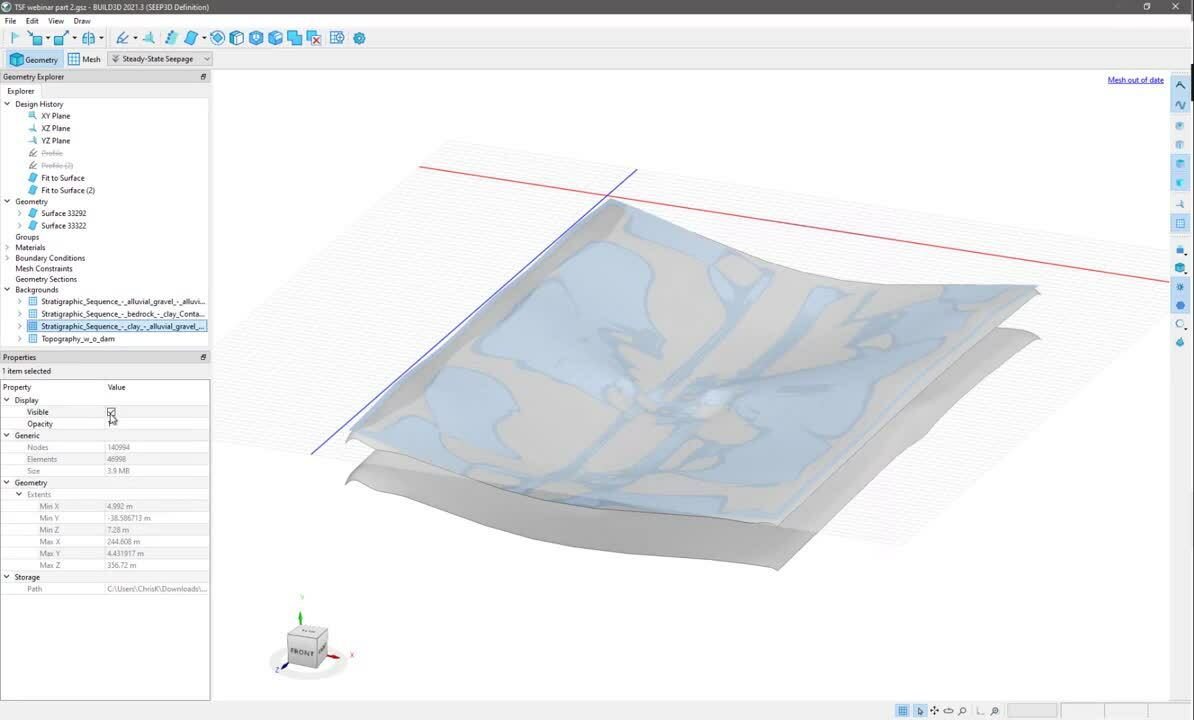
In GeoStudio, BUILD3D,

[00:09:11.920]
I have already imported a background mesh

[00:09:14.810]
for the topography of the site.

[00:09:21.838]
I’ll turn off the visibility

[00:09:23.650]
and navigate to import background from Central.

[00:09:28.820]
In this window, I select the Central server,

[00:09:33.540]
then the project name, then the branch,

[00:09:41.650]
the ID, and finally, the geological model.

[00:09:49.850]
After hitting okay,

[00:09:51.600]
I will navigate into the import background window

[00:09:56.800]
and change some of the key settings

[00:09:58.520]
to create these background meshes.

[00:10:02.210]
First off, notice I can select which background mesh

[00:10:05.560]
from the geological model I want to include in import.

[00:10:10.600]
Further down, we have a transformation section

[00:10:14.020]
of the dialog box.

[00:10:16.390]
Notice once the import is complete,

[00:10:18.760]
that the background meshes are not oriented

[00:10:21.590]
with the surface topography.

[00:10:23.960]
From the dropdown,

[00:10:25.260]
I can select a saved transformation.

[00:10:28.410]
This automatically remaps the axes

[00:10:30.700]
from Leapfrog coordinates to GeoStudio coordinates

[00:10:35.090]
and moves the base points such that the background meshes

[00:10:38.700]
are located closer to the 0-0-0 axes.

[00:10:51.080]
BUILD3D is a parametric modeling package.

[00:10:54.040]
As such, the background meshes need to be converted

[00:10:57.240]
to spline surfaces using the fit to surface tool

[00:11:00.750]
in BUILD3D.

[00:11:02.948]
The surface is selected from the geometry explorer window,

[00:11:06.610]
under the background meshes.

[00:11:09.320]
The visibility of the background meshes

[00:11:11.520]
can be toggled on and off in this view.

[00:11:14.360]
I will leave visible the surface representing the contact

[00:11:17.530]
between the bedrock and overlying clay unit.

[00:11:22.470]
With that done, the fit for surface icon is selected,

[00:11:26.300]
and three parameters are adjusted,

[00:11:28.540]
including the acceptable difference

[00:11:30.900]
between the background mesh and the spine surface,

[00:11:34.670]
the resolution, and a parameter controlling

[00:11:38.290]
the flexibility of the surface.

[00:11:41.100]
For this problem, I will adjust

[00:11:42.820]
both the resolution and the flexibility to 0.75.

[00:11:47.960]
Rotating the surface in space

[00:11:49.730]
reveals an acceptable fit

[00:11:51.740]
compared to the original Leapfrog surface mesh.

[00:11:58.870]
Next, I will turn off the visibility of the background mesh

[00:12:03.480]
and turn on the next stratigraphic layer,

[00:12:06.620]
repeating the process of using the fit to surface tool

[00:12:11.240]
on each occasion.

[00:12:13.150]
The process is repeated for each subsequent contact

[00:12:16.840]
along with the ground surface.

[00:12:19.530]
It is evident in the geometry explorer

[00:12:22.340]
that new surface bodies are added to the list

[00:12:25.360]
with each successive operation.

[00:13:08.730]
Now that the surfaces have been created,

[00:13:11.770]
I will unsuppress a sketch that I created

[00:13:14.440]
on the X-Z plane.

[00:13:17.160]
I will right click and edit this sketch

[00:13:19.280]
to demonstrate that I offset the plane for this sketch

[00:13:22.680]
in the y-direction, or vertical direction,

[00:13:25.870]
to ensure that it was located

[00:13:27.670]
beneath the lower stratigraphic surface in the domain.

[00:13:41.940]
The extrude icon is then selected

[00:13:45.420]
to push the profile upwards and generate a solid body.

[00:13:50.350]
I arbitrarily selected an extrusion distance of 150 meters

[00:13:55.700]
to ensure that the top of the block

[00:13:58.070]
far exceeds the ground surface elevation.

[00:14:07.100]
Clicking on the operation and the design history

[00:14:10.030]
reveals a single solid.

[00:14:15.010]
The cut tool is now used to turn the cube

[00:14:16.110]
into a geometry that is consistent with

[00:14:18.460]
the geological model in Leapfrog.

[00:14:21.530]
The cut operation that I select

[00:14:23.970]
removes the cutting tool,

[00:14:26.910]
which in this case are the surface bodies,

[00:14:30.400]
after the cutting operation is complete

[00:14:43.800]
Inspection of the resulting geometry

[00:14:46.410]
reveals a number of individual solids.

[00:14:49.880]
The delete body is used to remove

[00:14:52.950]
the upper most solid, leaving our four stratigraphic units,

[00:14:58.350]
to which I will assign a material.

[00:15:06.350]
The bottom most layer is assigned a bedrock material,

[00:15:12.630]
and then the overlying units in turn

[00:15:18.600]
include, clay, gravel, and aluminum.

[00:15:34.760]
Prior to the start of this webinar,

[00:15:37.280]
I imported an as-built design drawing

[00:15:40.630]
via the import body tool.

[00:15:43.870]
In the design history,

[00:15:46.090]
I will right click the profile and unsuppress.

[00:15:53.550]
The cross section of the downstream tailings dam

[00:15:56.580]
and tailings is now visible.

[00:16:05.520]
I’m going to click on the profile

[00:16:07.760]
and subdivide the tailings into a number of layers.

[00:16:13.490]
I’m doing this simply for the purpose

[00:16:15.750]
of conducting a geotechnical technical analysis.

[00:16:19.320]
For simplicity, I will split the tailings into five raises.

[00:16:26.150]
BUILD3D is a feature-based geometry creation tool,

[00:16:30.400]
so we can edit this sketch at any time

[00:16:33.150]
and all the changes are automatically cascaded

[00:16:36.460]
through the entire model’s geometry.

[00:17:29.656]
With the drawing complete, I will hit okay.

[00:17:32.270]
And the geometry is regenerated.

[00:17:37.390]
Notice that the as-built section

[00:17:39.450]
is located at the center line of the valley.

[00:17:42.750]
In preparation for an extrusion,

[00:17:45.260]
the location of the section needs to be offset.

[00:17:50.730]
Right clicking the profile and editing

[00:17:54.970]
reveals the original location of the plane end profile.

[00:18:01.660]
I can change the offset to sit inside the domain,

[00:18:05.540]
as shown.

[00:18:09.680]
This position moves the profile inside the ground surface.

[00:18:14.370]
It will become apparent when I extrude the profile

[00:18:17.780]
that our goal here is simply to ensure

[00:18:20.070]
that the geotechnical structure traverses the entire valley

[00:18:24.240]
in a manner consistent with the actual construction.

[00:18:46.449]
With the tailings dam profile

[00:18:47.960]
now located inside the upper ground surface,

[00:18:51.230]
I will right click the profile and select extrude.

[00:19:07.320]
The extrusion distance is arbitrarily set to 50 meters

[00:19:11.620]
and then 100 meters, causing the extruded profile

[00:19:16.180]
to span the entire valley.

[00:19:27.450]
Notice the shadow-like image that shows

[00:19:30.670]
the intersection between the structure

[00:19:33.570]
and the ground surface.

[00:19:57.890]
After rotating the camera angle,

[00:20:00.170]
I’m going to select the solids that represent

[00:20:02.330]
the tailings dam and create a group.

[00:20:10.940]
The material for this group of solids is then changed

[00:20:14.940]
and the process is repeated for the tailings layers.

[00:20:32.260]
We see the fill material listed in the drop down list.

[00:20:38.100]
And then, again, I’ll select these next five solids

[00:20:41.220]
for the tailings layers,

[00:20:43.810]
create the group and rename it.

[00:20:49.300]
Select the group

[00:20:51.400]
and then change the material type.

[00:21:06.630]
Clicking in the geometry explorer

[00:21:08.790]
reveals that the solids extend into the flanks

[00:21:12.770]
of the valley wall.

[00:21:14.930]
I therefore need to remove this portion of the tailings

[00:21:17.770]
and dam geometry using the cut tool.

[00:21:21.280]
In this case, the first and second stratigraphic units

[00:21:25.490]
are used as the cutting tool

[00:21:27.440]
and the option to remove the overlapping solids is selected.

[00:21:31.870]
Once the operation is completed,

[00:21:34.350]
I can select the upper stratigraphic layer

[00:21:37.260]
and note visually that the tailings structure

[00:21:39.960]
does not extend into it.

[00:21:51.540]
I do this by first toggling off the surface selection tool

[00:21:55.490]
and then selecting only solids.

[00:22:07.790]
At this point in the workflow,

[00:22:09.990]
the analysis ready geometry is complete.

[00:22:18.350]
We could now proceed to mesh the domain,

[00:22:21.690]
then return to the geometry definition,

[00:22:25.740]
apply boundary conditions, and then solve the analysis.

[00:22:41.200]
We can see now that the finite element mesh is complete.

[00:22:47.210]
I’m switching back to the geometry view,

[00:22:50.410]
selecting the surface of the tailings,

[00:22:55.240]
and applying a hydraulic boundary condition.

[00:23:04.570]
Conversely, we could create a two dimensional analysis

[00:23:09.160]
based on the 3D geometry and poor water pressure conditions.

[00:23:13.830]
To do this, I select the geometry section tool.

[00:23:19.090]
Once the location has been selected,

[00:23:22.970]
I can hit okay,

[00:23:27.030]
navigate down to the geometry sections area,

[00:23:30.710]
right click, and generate 2D GeoStudio geometry.

[00:23:37.880]
Closing BUILD3D and going back into GeoStudio,

[00:23:42.280]
we now see a 2D geometry in the analysis tree,

[00:23:46.500]
to which I will add a slope/w analysis.

[00:23:51.620]
Note that the materials are automatically mapped

[00:23:54.810]
to the regions.

[00:23:58.970]
Accordingly, I can click on define, materials

[00:24:04.180]
and the list of materials is populated

[00:24:07.120]
by simply defining a material model

[00:24:09.620]
such as Mohr-Coulomb,

[00:24:11.710]
we see the colors of the materials mapped to the regions.

[00:24:21.850]
Now we come full circle to the heart of the issue.

[00:24:24.900]
We have a 2D and 3D geotechnical analysis,

[00:24:28.560]
which together, with the geological model,

[00:24:31.250]
form a comprehensive digital twin.

[00:24:34.460]
As noted at the onset,

[00:24:36.430]
evolving site conditions and new data

[00:24:39.130]
could cause the geological model to change.

[00:24:42.800]
We need to ensure that the geotechnical analysis

[00:24:45.960]
is based on the most up-to-date site model.

[00:24:50.210]
In Leapfrog, the geological model

[00:24:52.780]
is dynamically updated by introducing new information,

[00:24:56.870]
such as geophysical data, polylines,

[00:24:59.720]
design drawings, and more.

[00:25:01.910]
For demonstration purposes,

[00:25:03.960]
let us simply assume that an error was observed

[00:25:07.360]
in the borehole data.

[00:25:13.940]
Notice that the stratigraphic layers

[00:25:15.587]
are not smooth and continuous in this profile.

[00:25:26.080]
I’m going to open the borehole log data

[00:25:28.850]
and alter the stratigraphic contact depths.

[00:25:40.240]
I’ll quickly do this by changing the depth to the contacts

[00:25:44.810]
in boreholes 10 and 12.

[00:26:19.710]
After saving the file,

[00:26:21.090]
I will reload the borehole data

[00:26:23.560]
and then reprocess the geological model.

[00:26:30.070]
So first, reload the boreholes.

[00:26:35.230]
Then, navigate to the play button on the top left

[00:26:46.200]
and select run all.

[00:26:53.380]
The geological model is updated

[00:26:55.750]
as indicated by the new, smoother geological contacts.

[00:27:08.630]
Looking at the slice from the backside

[00:27:11.050]
reveals nice, smooth, continuous contacts.

[00:27:16.700]
Then, rotating the camera view around to the front

[00:27:20.320]
similarly demonstrates that the geological model

[00:27:24.900]
has been updated.

[00:27:29.260]
After publishing the Leapfrog model to Central,

[00:27:32.210]
I can now return to GeoStudio

[00:27:34.680]
and reload the background meshes

[00:27:37.200]
used at the onset to create the analysis-ready geometry.

[00:27:43.120]
I do this by multi selecting three surfaces,

[00:27:46.940]
right clicking, and reloading.

[00:27:51.440]
We can see in the bottom right of the tray

[00:27:53.590]
that the Boolean operations are being recomputed.

[00:27:57.760]
This is a key advantage of a feature-based modeling package

[00:28:01.590]
like BUILD3D, because any change to the model

[00:28:05.290]
is automatically cascaded through the design history.

[00:28:09.990]
Once complete, we can switch over to the mesh view,

[00:28:14.670]
remesh the domain,

[00:28:17.370]
and then I will use the clipping tool

[00:28:19.920]
to inspect the updated geology.

[00:28:25.450]
The process takes just a couple seconds

[00:28:28.060]
to recompute all the contacts and update the model.

[00:28:33.350]
Again, the clipping plane tool,

[00:28:35.530]
much like a sectioning tool,

[00:28:37.300]
allows us to look inside the domain.

[00:28:40.270]
Notice that the contacts have all been updated

[00:28:43.430]
and they’re now nice and smooth.

[00:28:49.000]
With this new clipping plane,

[00:28:50.650]
I will change the camera view.

[00:28:54.880]
We see the clean geology and the new contacts.

[00:29:01.410]
Then I will navigate to the 2D geometry section

[00:29:07.260]
back on the geometry window.

[00:29:13.010]
First shutting off the clipping plane,

[00:29:17.110]
then switching back to geometry view,

[00:29:21.270]
scrolling down, selecting our section,

[00:29:25.710]
which runs down the center line of the valley,

[00:29:28.160]
I’ll right-click, generate a new section

[00:29:30.950]
which replaces the old section.

[00:29:33.860]
I can then close BUILD3D.

[00:29:36.620]
And back in GeoStudio,

[00:29:38.330]
when I click on the slope stability analysis,

[00:29:41.140]
we see the new geology are reflected

[00:29:43.990]
in this cross section.

[00:29:52.300]
In summary, teams have to think about

[00:29:54.700]
a holistic modeling approach

[00:29:56.660]
with the digital twin at its core

[00:29:58.990]
in order to manage tailing storage facilities safely

[00:30:02.170]
and consider the requirements

[00:30:03.650]
of the global tailing standard.

[00:30:06.780]
The digital twin becomes the basis for design

[00:30:09.970]
used at all phases of the project’s life cycle.

[00:30:13.500]
It invites the engineers to participate

[00:30:15.700]
in the investigation of the physical system,

[00:30:18.520]
to understand the geological constraints,

[00:30:21.350]
and make informed decisions about the facility’s

[00:30:23.730]
performance as it evolves.

[00:30:25.840]
A comprehensive and dynamically updated digital twin

[00:30:30.420]
consistently incorporates changing data

[00:30:33.270]
and evaluates all spatial, numeric,

[00:30:36.570]
and intellectual information in a 3D context.

[00:30:41.060]
It can also help design targeted monitoring programs.

[00:30:44.890]
Interpreting monitoring data is a significant challenge

[00:30:48.410]
as it goes beyond plotting a time series of data.

[00:30:52.670]
Again, data is only valuable if it is interpreted

[00:30:56.350]
in the context of the digital twin.

[00:30:59.770]
Thank you for your time and attention.

[00:31:01.870]
We look forward to welcoming you again

[00:31:04.270]
in mid-July for the third part of our webinar series.

[00:31:08.090]
Dr. Yanina Elliott will discuss an agile workflow

[00:31:11.440]
that accommodates stakeholder engagement.

[00:31:13.970]
This will bring together all the key components

[00:31:16.390]
of the Seequent ecosystem to demonstrate

[00:31:18.840]
how owners, analysts, engineers of record, and auditors

[00:31:23.460]
can collaborate on the management

[00:31:25.280]
of a tailing storage facility.

[00:31:27.760]
Thanks again, and have a great day.