Introduction

The temperature of underground pipelines can have a significant influence on the overall thermal regime of the surrounding soil. This influence can also be effected by the presence of groundwater flow. Understanding the thermal regime within the surrounding soil is important when considering the design and operation of pipelines. This example illustrates a conduction-only (TEMP3D) analysis of a chilled pipeline, as well as a coupled analysis (SEEP3D and TEMP3D) that considers the influence of groundwater flow on the thermal response of the surrounding soil.

Numerical Simulation

The soil foundation in this example is represented by a three-dimensional rectangular domain that is 30 m long and 20 m wide, with a depth of 10 m (Figure 1). A cooling pipe can be seen cutting through the soil domain with an S-shaped curve. The global element mesh size for the 3D geometry is set to
0.5 m. The mesh surrounding the pipeline was refined with a mesh constraint of 0.1 m applied to the pipe surface.

There are three analyses in the project file (Figure 2). The first analysis is a steady-state hydraulic and thermal analysis, which determines both water and heat transfer over the project domain. These results provide the initial temperature and pore-water pressure conditions for the following two transient analyses. The first transient analysis considers conduction-only when simulating the thermal response of the foundation to the cooling pipe. The second transient analysis includes water transfer physics in order to consider the influence of groundwater flow on the overall thermal regime.

The duration of both transient analyses must be changed to 200 days, with 600 time steps that increase exponentially from an initial time increment of 0.5 hours (Figure 3). The results are saved every 480 steps to reduce solve time. Several time steps are specified (10, 20, 40, 80, and 120 days) such that they appear in the defined time steps.

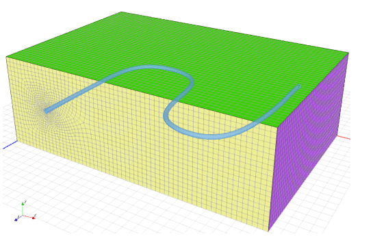
Figure 1. 3D geometry with an S-shaped pipeline.

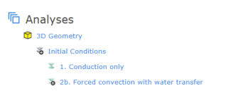
Figure 2. Analysis tree for the project file.

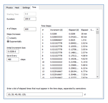
Figure 3: Time increment definition for the two transient analyses (in the Define Project dialogue).

The Full Thermal Material Model is used in all three analyses to define the thermal properties of the silty sand foundation. The thermal conductivity function is estimated using the silty sand material type, with a frozen thermal conductivity of 3.241 x 10-3 kJ/s/m/⁰C, and an unfrozen thermal conductivity of 1.505 x 10-3 kJ/s/m/⁰C (Figure 4). The normalized unfrozen volumetric water content function is also estimated using the silty sand material type (Figure 4). The volumetric heat capacity is set to 2100 kJ/m3 /⁰C, and the volumetric water content is 0.3.

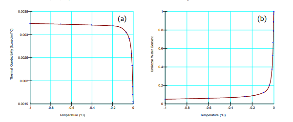
Figure 4. Thermal conductivity function (a) and normalized unfrozen volumetric water content function (b) for the Silty Clay material.

The saturated/unsaturated hydraulic material model is used for the water transfer analyses. The “Reduce Conductivity in Frozen Ground” option is selected to ensure that frozen conditions are associated with a decrease in hydraulic conductivity. The volumetric water content and hydraulic conductivity functions are shown in Figure 5.

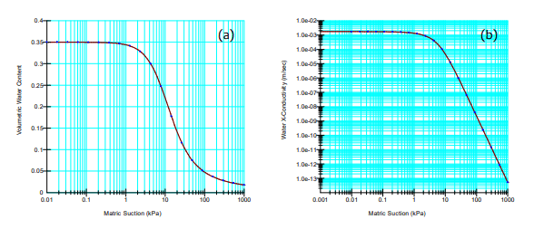
Figure 5. Volumetric water content (a) and hydraulic conductivity (b) functions for the silty sand material.

All three analyses have the same thermal boundary conditions applied on the upper and lower boundaries of the domain. Constant temperatures of 12⁰C and 5⁰C have been applied to the ground surface and bottom boundary, respectively. A temperature function was applied to the perimeter of the pipe in the two transient analyses, to represent the cooling of the pipeline over a period of 5 days. The temperature decreases from 9⁰C to -2⁰C and then remains constant for the remainder of the time steps (Figure 6). The hydraulic boundary conditions applied to the steady-state and forced convection analyses include total head boundary conditions of 6.00 m and 6.02 m, applied to opposite sides  of the domain to generate constant lateral water flow.

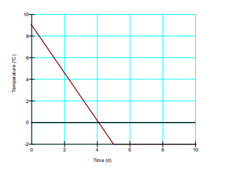
Figure 6. Cooling temperature function representing the temperature in the cooling pipeline.

Results and Discussion

When groundwater flow is not considered, the soil surrounding the cooling pipeline slowly decreases in temperature over the duration of the transient analysis (Figure 7). In the second transient analysis with groundwater flow, the location of the freezing front changes. The temperature at the midpoint between the pipes, at an elevation of 5 m, drops to around 5⁰C in the initial 40 days, and then continues to slowly decrease over the remainder of the analysis. The temperature decrease after 40 days is more substantial for the midpoint at x = 10 m. This is because groundwater passing this location is cooled by two sections of the pipe, while the groundwater passing the x = 20 m location has only been cooled by one section of the pipe.

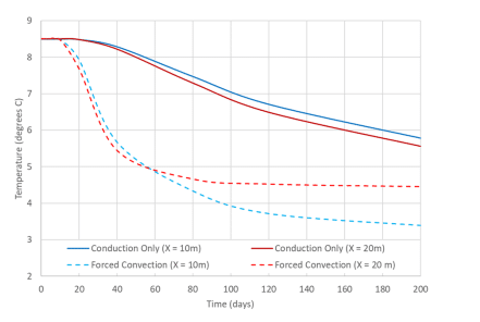
Figure 7. Temperature over time at the midpoints between the curved sections of the pipeline (at 5 m elevation).

Temperature isosurfaces help to visualize the change in the thermal regime when groundwater flow is simulated. The freezing front around the pipeline reaches an approximate diameter of 1.5 m in the conduction-only analysis (Figure 8). The isosurfaces around each section of the cooling pipe are symmetric about a vertical axis as illustrated in Figure 8. In the forced convection example, propagation of the freezing front is minimal on the upstream side of the cooling pipeline (Figure 9). Instead, the freezing front propagates further in the downstream direction due to the effects of groundwater flow. Interestingly, the freezing front propagation in the downstream direction is greatest for the section of pipe that is furthest downstream (i.e. the section on the far left of Figure 9). This corresponds to the temperature over time trends (Figure 7), which indicate a greater temperature drop for the location that was further downstream.

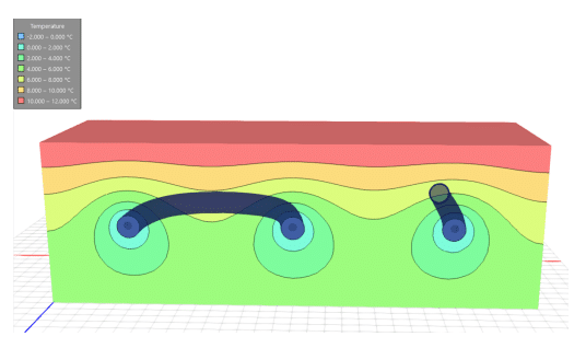
Figure 8. Temperature contours on the plane at z = 10 m for the conduction-only analysis after 200 days.

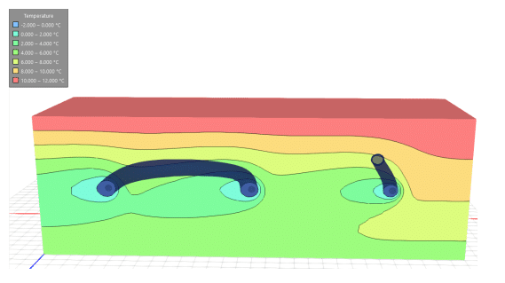
Figure 9. Temperature contours on the plane at z = 10 m for the forced convection analysis after 200 days.

The temperature along a polyline parallel to the x-axis at y = 5 m and z = 10 m (Figure 10), confirms the effects of groundwater flow indicated by the temperature isosurfaces. In the conduction-only analysis, the temperature variation is similar between the locations where the polyline intersects the pipeline (at 5, 15, and 25 m). The forced convection analysis results illustrate the downstream propagation of the pipe’s cooling effect.

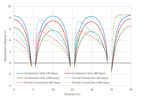
Figure 10. Temperature along a polyline parallel to the x-axis, at y = 5 m and z = 10 m, at varying time steps.

Temperature profiles at multiple time steps were plotted on two vertical polylines at x = 10 m, z = 10m, and x = 20 m, z = 10 m (Figure 11). As expected, the profiles from the conduction-only analysis were similar at both locations. The forced convection analysis results confirm that groundwater flow causes greater cooling of the soil profile further downstream.

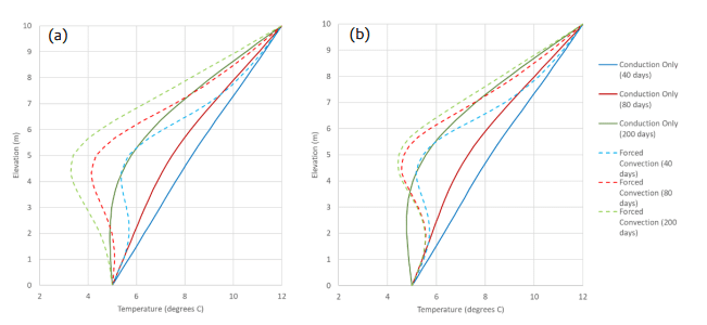
Figure 11. Temperature profiles at three time steps for polylines at x = 10 m, z = 10 m (a) and x = 20 m, z = 10 m (b).

Summary and Conclusions

This example illustrates the use of three-dimensional thermal and hydraulic analysis to investigate freezing front propagation from an S-shaped pipeline. Two scenarios were simulated, one with heat transfer via conduction-only and the other with heat transfer via conduction and forced convection. The inclusion of groundwater flow demonstrated the influence of water transfer on the thermal regime within the soil surrounding the pipeline.