Find the best drilling target using Leapfrog Geothermal

(our add on geostatistical module) and determine the best drilling target for your next deep geothermal well.

This presentation introduces a new and modern workflow for 3D data integration using a Play Fairway Analysis approach, using various sub-surface datasets from geology to geophysics and well data. You’ll learn how to combine them into a single calculated model that highlights the most promising areas for drilling.

Overview

Video Transcript

[00:00:01.536](soft upbeat music)

[00:00:09.940]<v ->Welcome to today’s webinar.</v>

[00:00:12.050]My name is Bastien Poux.

[00:00:13.190]I am the Technical Sales Advisor for energy at sequence,

[00:00:16.630]based out of Vancouver in Canada.

[00:00:20.410]During this webinar,

[00:00:21.300]I will show you a new workflow

[00:00:22.920]to help you find the best drilling target or targets

[00:00:25.930]for your geothermal project

[00:00:27.750]using Leapfrog Geothermal and Edge.

[00:00:30.530]Please note that this is a technical webinar,

[00:00:34.027]but the technical aspect of it is quite advanced,

[00:00:37.610]although it does not require any specific knowledge

[00:00:40.460]of Leapfrog Geothermal or Edge,

[00:00:43.540]but some background in geothermal resource exploration

[00:00:46.330]and the main concepts of geo modeling,

[00:00:49.460]will definitely be helpful to better understand the workflow

[00:00:52.110]that I’m going to present.

[00:00:57.670]So here is a short agenda where we’re going to see today.

[00:01:02.200]So I would start with an explanation

[00:01:04.150]of the conceptual approach we took for this workflow,

[00:01:07.880]as well as tools and the data

[00:01:10.840]that were used to develop it.

[00:01:13.610]Then we will look at the different steps

[00:01:16.070]involved in the methodology.

[00:01:18.290]And we’re going to look at the results

[00:01:20.160]and see how to plan a new direction or well

[00:01:23.130]based on those results.

[00:01:24.980]Finally, after a short conclusion,

[00:01:26.990]I will have some time to address some of the questions.

[00:01:31.744]I expect we’ll have about 10, 15 minutes

[00:01:33.130]for a good Q&amp;A session.

[00:01:36.950]So the workflow I will present today

[00:01:39.600]is based on the well established technique,

[00:01:41.770]called the Play Fairway Analysis or PFA.

[00:01:44.850]Which you might have heard before in a variety of context.

[00:01:48.620]Play Fairway Analysis,

[00:01:50.107]they have long been utilized in the hydrocarbon industry

[00:01:53.000]to mitigate explorationist from a regional

[00:01:55.820]to a prospect global scale.

[00:01:58.530]And more recently, we have seen this methodology

[00:02:01.360]that has been used in the geothermal industry too,

[00:02:04.740]which will really consist in series of studies

[00:02:07.050]in the USA mostly, but also more recently international.

[00:02:13.600]So it ended up in a Play Fairway Analysis,

[00:02:17.380]the main concept is to use various parameters

[00:02:21.730]in favor of the presence of a geothermal resource

[00:02:24.820]and to classify them, to weight them,

[00:02:27.300]and to combine them together.

[00:02:29.780]So this process can be more less complex

[00:02:33.100]based on the data available.

[00:02:34.320]And the methodology keeps being improved over the years.

[00:02:39.220]The results of a Play Fairway is a special distribution

[00:02:43.360]of the geo for more resource favorability.

[00:02:46.410]It is generally used to focus richer exploration work

[00:02:51.160]in the most suitable areas.

[00:02:53.110]So we have two examples here on the right.

[00:02:56.240]The one at the top is the Play Fairway

[00:02:58.600]that was done in Hawaii.

[00:03:01.416]And you can see on the left a little diagram explaining

[00:03:04.860]which data are considered, how they were classified

[00:03:08.160]and combined together to create this favorability map.

[00:03:13.840]The one below is a bit more complex,

[00:03:16.290]and it’s a study looking at about the Port of Nevada

[00:03:20.890]in the U.S.

[00:03:22.070]You can see that there’s a lot more data

[00:03:24.030]that were considered, and that the general classification

[00:03:28.540]and combination process is a lot more advanced,

[00:03:31.610]but the result is the same.

[00:03:32.740]We get at the end a Play Fairway map

[00:03:36.480]that indicates the most favorable area

[00:03:39.030]for geothermal exploration.

[00:03:42.300]So this type of study has mostly being completed

[00:03:45.130]in two dimensions in the past,

[00:03:46.730]like we just saw in those maps,

[00:03:48.510]using GIS type of mapping application

[00:03:51.770]and using surface data.

[00:03:53.810]The new approach I will present today establishes a workflow

[00:03:57.490]to complete a Play Fairway Analysis,

[00:03:59.740]but in three dimensions.

[00:04:01.530]So it is based on the existence of enough

[00:04:03.593]types of surface data

[00:04:05.750]obtained for a project during exploration, during drilling,

[00:04:08.380]during laboratory analysis of samples,

[00:04:12.930]also reservoir testing, and more.

[00:04:16.600]So we often talk about data integration

[00:04:19.340]to understand the resource.

[00:04:20.860]And Leapfrog Geothermal is being used widely in the industry

[00:04:24.180]to visualize any temperate all data in 3D

[00:04:27.160]and to observe the special relations,

[00:04:29.920]to better understand the geothermal resource.

[00:04:32.870]But as we know, the human mind sometimes interpret data

[00:04:36.730]with some degree of bias and is prone to mistakes.

[00:04:41.200]So this is why by applying a computerized technique,

[00:04:44.740]we are eliminating this human behaviors

[00:04:47.280]and we get more accurate results

[00:04:49.230]and we lower even more the risk associated

[00:04:52.730]with geothermal exploration.

[00:04:57.330]So the workflow today, what we’re going to to do is,

[00:04:59.210]we’re going to combine some geological data,

[00:05:02.170]silotologies and structure, some geophysical data,

[00:05:06.010]as well as some data obtained from the wells

[00:05:10.290]in order to find where would be the best drilling target

[00:05:13.870]or targets for future geothermal deep well.

[00:05:18.100]So the results of the Play Fairway Analysis

[00:05:19.950]will be a single calculated three dimensional model

[00:05:24.790]that shows the most favorable area

[00:05:26.990]for the presence of a geothermal reservoir.

[00:05:29.330]And consequently, indicating the best targets for drilling.

[00:05:34.510]I will introduce very quickly the tools we’ve used.

[00:05:38.320]So the main tool we use is sequenced software

[00:05:41.320]called Leapfrog Geothermal.

[00:05:43.130]So a Leapfrog Geothermal is a workflow based

[00:05:46.160]3D geological modeling tool using implicit modeling engine.

[00:05:51.660]So Leapfrog creates workflows

[00:05:54.250]between a member of the resource team

[00:05:57.840]and brings all the geoscientific data

[00:06:00.230]in a single 3D environment.

[00:06:02.660]It also integrates with reservoir engineering

[00:06:05.450]and geophysical modeling software.

[00:06:09.630]It is based on a proprietary algorithm

[00:06:12.570]called the fast radial basis function,

[00:06:15.290]which allows for fast processing, dynamic updating,

[00:06:18.370]which means that when you integrate new data,

[00:06:21.300]the models will automatically update and adapt.

[00:06:25.050]And this allows you to test multiple scenarios.

[00:06:31.670]In addition to Leapfrog Geothermal,

[00:06:33.890]we have used a module that goes with it

[00:06:36.810]that’s called Leapfrog Edge.

[00:06:38.950]Edge originally was developed for the mining industry.

[00:06:42.270]And it was recently adapted

[00:06:44.420]to be used in geothermal as well.

[00:06:47.700]It combines advanced geo statistical tools

[00:06:50.470]and resource estimation tools.

[00:06:53.380]And one of its feature, which is key to the workflow

[00:06:57.980]I’m presenting today

[00:06:59.240]is that it allows you to make calculations on the data.

[00:07:05.530]The geothermal project that we’ve used to develop

[00:07:09.020]this workflow that I’m going to use today during this webinar

[00:07:11.950]is a synthetic model.

[00:07:13.500]So it was developed specifically for research proposals

[00:07:16.970]and represent a geothermal system.

[00:07:20.300]It is highly inspired by geothermal fields in New Zealand.

[00:07:24.533]Sequent is a company based in New Zealand.

[00:07:28.990]And in terms of geology and resource characteristic,

[00:07:32.040]it’s quite similar to the fields that we find there,

[00:07:35.210]but the workflow, ’cause our work could be applied

[00:07:37.760]to any other geological context as well.

[00:07:40.620]And from low to high temperature geothermal fields.

[00:07:45.340]So we have integrated datasets and build models

[00:07:49.890]that can be grouped based on the information they provide

[00:07:53.470]which will get to the geothermal resource.

[00:07:56.340]Note that some of these models

[00:07:58.120]actually can provide information

[00:07:59.750]for more than one element of the resource.

[00:08:02.220]Here I’m just introducing the models

[00:08:04.950]based on what information they bring.

[00:08:07.880]But this is not the classification

[00:08:09.400]that we use in the Play Fairway Analysis.

[00:08:11.880]This is just a way for me to introduce you

[00:08:14.050]to the different models.

[00:08:18.290]So we consider that these models that I’m talking about here

[00:08:22.730]have previously been built in Leapfrog Geothermal,

[00:08:25.990]and in this webinar I’m not going to show you

[00:08:28.917]how they were built,

[00:08:30.860]but if you have questions about the modeling tools,

[00:08:33.880]please feel free to reach out

[00:08:35.550]and I would be happy to provide you with some information.

[00:08:39.860]So I will introduce the models

[00:08:41.310]and then we’re going to see them in 3D directly.

[00:08:45.190]So their Natural State Temperature model

[00:08:47.850]and the Alteration mineralogy model,

[00:08:50.170]they both provide some good information

[00:08:52.040]about the distribution of heat in the subsurface,

[00:08:55.290]which as you know, is a critical element

[00:08:58.130]for the presence of geothermal resource.

[00:09:00.700]Now, if we look at the structural data,

[00:09:03.565]the lithological model also, the lithologies,

[00:09:06.530]the seismicity, were about the distribution of earthquakes

[00:09:10.020]and where the food entries are located in the existing well,

[00:09:13.810]this also gives you information

[00:09:15.520]about the permeability distribution in the sub surface.

[00:09:19.600]In some measure, the empty model, the magnetotelluric model

[00:09:23.540]can also provide some information about permeability.

[00:09:28.510]And finally we have,

[00:09:30.204]so the empty magnetotelluric resistivity model

[00:09:33.660]and the Alteration mineralogy model,

[00:09:36.020]which can give you information about the location

[00:09:39.470]and the size of the clay cap or seal

[00:09:43.270]that is located above the geothermal reservoir.

[00:09:49.300]And because in this study,

[00:09:51.360]we are looking at finding the best drilling target.

[00:09:53.930]We have also considered some drilling constraints.

[00:09:56.630]So we will also have a model of the depth

[00:10:00.880]because as you know, the cost of drilling increase

[00:10:04.420]with the depth we are drilling to,

[00:10:07.100]and we also going to integrate

[00:10:11.350]the location of the existing wells

[00:10:14.191]and do a distance ’cause we want to avoid drilling too close

[00:10:17.440]to an existing well.

[00:10:20.580]So on the right here, you see a conceptual model

[00:10:23.350]that regrouped the most important information

[00:10:26.370]for this field.

[00:10:27.840]And this is what usually the geothermal resource team

[00:10:32.600]will use to select the drilling target.

[00:10:34.860]But this is actually where this new workflow just starts.

[00:10:39.520]So I’m going to go through these different models now.

[00:10:45.800]So first we have a simple geological model,

[00:10:49.110]so you can see there are different lithologies.

[00:10:52.820]The basement here in gray, we have,

[00:10:55.750]but five faults intersecting each other with a fault offset.

[00:11:00.530]So this was built mostly using the well data

[00:11:06.210]and also a surface geological map and some interpretation.

[00:11:16.990]We also have the Alteration mineralogy model.

[00:11:20.050]So this represents the different types

[00:11:23.096]of Alteration minerals presence in the resource.

[00:11:25.840]In yellow here is a important one epidote

[00:11:28.700]which indicates the beginning of the geothermal reservoir

[00:11:32.910]because it usually forms a temperature

[00:11:34.890]above 220 degrees celsius.

[00:11:37.820]But in brown is also here an important mineral,

[00:11:41.700]which is uses smectite as it composed most of the clay cap

[00:11:46.030]above the reservoir.

[00:11:49.640]Now we’re going to look at the temperature model

[00:11:52.590]that was built.

[00:11:53.750]So this shows the temperature distribution

[00:11:57.540]in the strips surface.

[00:11:58.600]It’s based on interpretation

[00:12:00.540]and on a temporary logs in the well.

[00:12:07.260]Same, see the Wells and the temperature low along the wells,

[00:12:12.000]and how the model looks creative.

[00:12:16.050]In terms of geophysical data,

[00:12:18.730]one of the most commonly used method in geothermal

[00:12:22.610]is magnetotellurics,

[00:12:24.250]and it gives you a 3D models of the resistivity

[00:12:28.080]in the subsurface.

[00:12:29.130]So he is an example of a empty model

[00:12:32.260]that we’re going to use in this project,

[00:12:35.200]and we can slice through it.

[00:12:38.060]And what you can see here is the highest conductivity,

[00:12:44.810]lower resistivity area here,

[00:12:47.220]which might well correspond to the clay cap

[00:12:50.650]above the reservoir.

[00:12:51.860]So we know that this is a promising area for geothermal.

[00:12:58.950]What about types of that data include seismicity data.

[00:13:02.080]So location of the earthquake.

[00:13:04.410]So here you recognize you are the force

[00:13:05.690]from the geological models,

[00:13:07.070]and you can see the locations of the earthquake ,

[00:13:11.300]they are colored and sized by magnitude.

[00:13:14.430]You can see that some of them align here

[00:13:16.330]with some of the faults.

[00:13:20.837]Other information we have on the wells include,

[00:13:25.120]well, the casing is here, but it’s not included.

[00:13:27.770]We’re not using it in the survey,

[00:13:30.100]but we can see that there are different fluid entries

[00:13:33.950]in the wells, small, medium, or large

[00:13:36.710]that we can also use in the analysis.

[00:13:40.950]And finally, I’ll talk about the draining constraints.

[00:13:44.290]This is just a depth model.

[00:13:45.880]So it’s a projection of the topography at depth,

[00:13:48.920]and I represents a depth you would have to drill too.

[00:13:59.150]All right, so once we have this model in our project files,

[00:14:08.740]we will have start looking at the workflow itself.

[00:14:11.400]So the workflow can be divided in four main steps.

[00:14:16.190]Right now we are at the top.

[00:14:18.480]So we have integrated all the data in 3D.

[00:14:21.930]And the first step will consist in preparing

[00:14:24.970]and integrating some of those models.

[00:14:28.640]Not all of them are already in a format

[00:14:31.210]that can be used in the analysis.

[00:14:34.068]Once those model are ready,

[00:14:36.720]we will evaluate them on what we call a Block model,

[00:14:40.010]which is a tool in Leapfrog

[00:14:41.710]that I would explain in a moment.

[00:14:43.390]So this step is necessary

[00:14:45.300]to be able to run calculations on the data.

[00:14:48.560]Step three, consists in what we call

[00:14:51.130]the categorization of the model.

[00:14:53.240]So we will create,

[00:14:54.370]will transform those models into index models,

[00:14:57.950]where we’re going to assign them favorability values

[00:15:01.030]from zero to five.

[00:15:03.760]So this step transforms the model into a similar format

[00:15:07.650]before the calculations.

[00:15:09.600]And finally, in the step four,

[00:15:11.710]we’re going to weight each of these index model,

[00:15:14.440]and we’re going to create the final 3D favorability model

[00:15:17.860]by combining them together.

[00:15:20.560]In the future,

[00:15:21.393]if we want to integrate more model in this analysis,

[00:15:24.400]they would have to go through each of these four steps

[00:15:27.570]before being integrated in the final calculation.

[00:15:34.570]So, as I mentioned in the previous slide,

[00:15:37.870]the first step is for some of the data,

[00:15:39.960]the data of models we need to first prepare them

[00:15:42.620]or interpret them.

[00:15:44.860]So I will list those models

[00:15:46.150]and then I will show those models directly.

[00:15:48.690]So the seismicity analysis you can see on the right

[00:15:52.550]on those three images consisted in combining

[00:15:55.620]the earthquake density with their magnitude.

[00:15:58.320]So those are the two elements that are important

[00:16:00.960]when looking at seismicity.

[00:16:04.210]Where there are the arrow

[00:16:05.570]that’s where we have a lot of earthquakes,

[00:16:07.420]and where the biggest of quakes happening.

[00:16:12.370]So this by itself is kind of a specific workflow in Leapfrog

[00:16:15.780]that that will not detail today,

[00:16:17.640]but if you are interested in this type of work, also,

[00:16:20.260]please, please get in touch.

[00:16:25.540]Now, the second types of data that we’re going to modify

[00:16:30.330]is the faults or faces, the fault intersections,

[00:16:34.160]which are lines.

[00:16:36.570]And the well traces which are lines also.

[00:16:38.700]So we need to convert those objects into volumetric objects,

[00:16:43.350]to be able to use them in the calculation.

[00:16:46.470]And for that, we will use what we call

[00:16:47.950]the distance analysis.

[00:16:51.505]Also, the magnetotelluric resistivity model.

[00:16:54.880]So it’s hard to directly relate a resistivity value

[00:16:58.750]to what it means in term of geothermal reservoir.

[00:17:02.000]So what needs to be done first,

[00:17:03.870]is to interpret the resistivity distribution

[00:17:07.550]in terms of very low, to very high favorability

[00:17:11.700]to geothermal resource.

[00:17:14.850]And finally, the fluid entries in the wells

[00:17:17.890]in order to highlight the most important,

[00:17:21.460]the biggest productive zones.

[00:17:25.490]We will use the square of the value of the fluid entry.

[00:17:33.060]And we’re going to divide that by this F analysis.

[00:17:35.700]So this is a workflow also that was used

[00:17:38.820]to integrate the fluid entries.

[00:17:44.080]So I’m going to explain what were those distance analysis.

[00:17:48.310]So here the three files I just mentioned.

[00:17:50.100]So the fault surfaces,

[00:17:51.920]the red lines are the fault intersections,

[00:17:54.560]and here we can see also the different wells.

[00:17:58.870]So when we do a distance analysis, for example,

[00:18:03.380]for the fault section is going to create for each point

[00:18:07.300]in space, a distance from any of these fault intersession.

[00:18:13.400]So here we can see, for example,

[00:18:14.770]the 500 meters and 1000 meter from the fault intersection.

[00:18:20.330]So he transforms a line into a 3D volumes.

[00:18:24.470]The same was done for the fault.

[00:18:26.200]So you can see here,

[00:18:27.033]we’re creating distances from the fault.

[00:18:29.750]And the further away we get a point here on the right,

[00:18:32.730]we’ll have a new unique value

[00:18:34.700]distance to whichever is the closest fault.

[00:18:39.039]And the same was done for the well traces.

[00:18:44.010]So we see here a buffer around the well traces.

[00:18:48.090]Right now, it’s going above the topography,

[00:18:49.810]but this will be cut during the calculation.

[00:18:53.310]So this top part will disappear.

[00:19:01.570]Now for the magnetotelluric, this one that I showed earlier,

[00:19:06.240]I mentioned that this high conductivity area above

[00:19:11.180]in this top part here,

[00:19:12.710]indicate the presence of the clay cap.

[00:19:15.740]So what do we did in this one is,

[00:19:17.980]we use different information.

[00:19:19.340]Here is a higher resistivity area.

[00:19:22.520]And this might mean that, you know,

[00:19:24.320]there are some fractures, some higher permeability.

[00:19:28.080]So this model was converted into different zones

[00:19:32.480]that would imitate that 3,500 meter,

[00:19:34.660]which is the limit of the analysis that we’ve done.

[00:19:38.030]And we created some areas from very low

[00:19:40.800]to very high favorability

[00:19:42.640]based on our interpretation of the entry data.

[00:19:45.210]So this is because we cannot directly use

[00:19:48.257]the resistivity values in our analysis,

[00:19:51.240]we have to first interpret the empty model.

[00:19:56.950]And finally the fluid entries.

[00:19:58.370]So this is the distance analysis around the fluid entries.

[00:20:02.840]And then we will do the the square

[00:20:05.960]of these prediction values that you see here

[00:20:08.490]and divide that by the distance analysis.

[00:20:10.250]I will show you the results later.

[00:20:15.260]So in total, we have 10 different models or data sets.

[00:20:21.270]And the step number two is to take all these models

[00:20:25.970]that were prepared

[00:20:27.030]and to project them on what we call a Block model.

[00:20:29.620]So a Block model is a tool in Leapfrog

[00:20:34.330]that allows you to run calculations on the model.

[00:20:38.209]It is a set of blocks and the user defines the dimension.

[00:20:41.860]Here we are using regular cubes of a hundred meters sides

[00:20:46.370]And what do we do is we take each of the 10 model

[00:20:49.300]and we’re going to project them on this grid

[00:20:53.550]to obtain a model like you can see on the right.

[00:20:57.980]So if we take this lithological model

[00:21:00.890]that is made of volume and surfaces,

[00:21:03.660]we project it on this Block model.

[00:21:06.360]So you can see the little blocks here.

[00:21:08.900]And we obtain this evaluation,

[00:21:11.480]a conversion of volumes and surfaces into little blocks.

[00:21:16.130]The advantage is that each of the block

[00:21:18.330]is assigned a unique value,

[00:21:20.390]whether it is a model with a numeric values like temperature

[00:21:23.980]or a model with categories like lithology,

[00:21:27.310]it will assign a single value per cube.

[00:21:34.900]So when we look at the different models,

[00:21:36.580]once they are being evaluated on the Block models.

[00:21:38.940]So this is the first one

[00:21:39.900]that I just showed in the previous slide.

[00:21:42.600]So it’s the lithology model,

[00:21:45.230]and we can look at other models.

[00:21:47.030]So the same way we have the alteration model,

[00:21:52.560]we also have this empty favorability model,

[00:21:58.350]the distance to the fault.

[00:22:00.520]So if I add the fault for the intersection,

[00:22:03.270]so this is a distance to the fault intersection.

[00:22:09.000]We also have the distance to the fault.

[00:22:12.540]So you see the red is the closest area to any fault.

[00:22:17.180]And then the further away

[00:22:18.170]the color changes to green and blue.

[00:22:25.310]We also have the temperature.

[00:22:32.090]We also had the distance to the well traces.

[00:22:34.470]So you can see here the distance further from a well,

[00:22:37.450]so the same goes above the topography,

[00:22:42.950]but this will cut later in the analysis.

[00:22:46.290]And we can also look at the model

[00:22:49.340]that shows the fluid entries.

[00:22:51.020]So if I add the fluid entries here,

[00:22:53.200]we see that it created the distance

[00:22:57.180]that will be around the prediction zones.

[00:22:59.750]And if it’s small producing zones,

[00:23:02.480]then the value will be lower

[00:23:05.080]than if it’s a high producing zone,

[00:23:06.920]it will get a higher value.

[00:23:13.168]And I think those are most of the models.

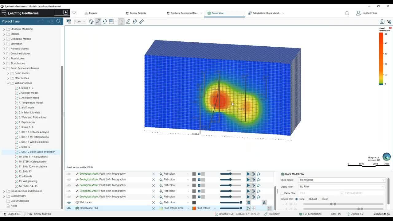
[00:23:22.940]So once we have evaluated all this model

[00:23:26.150]on the Block model…

[00:23:28.950]There’s something I want to show you here.

[00:23:31.560]So any block that we click in this Block model,

[00:23:35.540]so if I click on this little block here,

[00:23:37.370]you see that for each of the models that were evaluated,

[00:23:40.260]there is a unique value.

[00:23:43.360]So this one depth model is 2000, we’re in the (indistinct),

[00:23:48.750]low favorability for the empty.

[00:23:51.170]This distant to the fault, the average in this block

[00:23:53.950]is about 1.1 kilometer, et cetera, et cetera.

[00:23:57.310]So there is one unique value per block in this model

[00:24:00.660]for each of the model evaluated.

[00:24:05.420]So once we have all this model evaluated on the Block model,

[00:24:09.620]we have the possibility to start running calculation,

[00:24:12.520]to apply filters, and to do conditional queries

[00:24:16.620]using the Leapfrog Edge tools in Leapfrog.

[00:24:21.186]In this first step…

[00:24:22.937]In this first step sorry,

[00:24:23.860]we will assign index value for each category.

[00:24:27.150]When it’s a category model like lithology or alteration,

[00:24:31.340]we will select the different units and assign them a value.

[00:24:36.980]When it’s numeric models like temperature

[00:24:39.950]or distance analysis,

[00:24:42.260]we will create intervals to assign them an index value.

[00:24:46.880]The lowest value will be zero

[00:24:48.510]and the highest for the highest favorability will be five.

[00:24:51.940]And this would create what we call index models.

[00:24:56.320]So if I look at some of them in the table, for example,

[00:24:58.870]the distance to the fault from zero to a hundred meters,

[00:25:03.060]we are close to a fault.

[00:25:04.230]So it’s a better favorability.

[00:25:06.810]And the further away we get from the fault,

[00:25:09.580]the lower the favorability.

[00:25:11.250]And when it goes beyond 1.5 kilometers,

[00:25:15.530]then we assign a value of zero.

[00:25:17.710]For models with categories like the ethological model,

[00:25:20.670]or the alteration model we define by type of mineral value.

[00:25:25.110]So epidote, actinolite are high temperature minerals.

[00:25:29.760]So we assigned them values of four and five.

[00:25:35.360]How is that done in Leapfrog?

[00:25:38.250]So in the Block model, we can run all types of calculations.

[00:25:43.030]So those are the different tools available.

[00:25:47.010]So you can do addition, subtraction, testing,

[00:25:51.390]you can keep values to the minimum, maximum, et cetera.

[00:25:55.420]And here we have the different models that we evaluated.

[00:26:00.020]So for example, for the geological model,

[00:26:03.637]we’re going to use the conditional queries if and otherwise.

[00:26:07.640]So if the geological model is sediments,

[00:26:12.010]then we have this value of one.

[00:26:13.680]If we are in the basement, we gave the value of five.

[00:26:17.180]So those are the values from the table I showed before.

[00:26:21.100]Now, if we are looking at the distance from the fault,

[00:26:25.590]the same values as the table,

[00:26:27.290]if we are between zero and 50 meter,

[00:26:29.930]then we gave the value of five, et cetera, et cetera.

[00:26:39.640]What does it look like in 3D?

[00:26:43.080]So this is, you see the red on the right from zero to five,

[00:26:47.330]and this will show, so zero for this part,

[00:26:50.840]one here, two, et cetera.

[00:26:53.170]And we can look at the other model.

[00:26:54.960]So the full distance index also now only showing

[00:26:59.110]instead of a continuous current showing only values

[00:27:02.220]of five, four, three, two, and one and zero.

[00:27:05.430]And this will be the same for each of the model.

[00:27:07.970]Temperature, in temperature we created intermediate values.

[00:27:12.220]So one, 1.5 to 2.5, because that’s also a possibility.

[00:27:17.170]If you want to be more precise in your intervals,

[00:27:20.330]you also can create more intervals and get more precise.

[00:27:25.200]So this is the temperature model,

[00:27:26.640]index model for this project.

[00:27:31.490]We can look at the drilling.

[00:27:32.470]So of course the deeper we go, the lower is the index value.

[00:27:41.850]Distance from well, so lower value closer to the well trays,

[00:27:47.300]but then when we get started from the well,

[00:27:49.170]then we get the maximum value

[00:27:51.160]because there’s no risk of interference.

[00:27:56.010]Same for the resist interpretation,

[00:27:57.870]high favorability area, value of five in the middle.

[00:28:00.970]And where the favorability was lower

[00:28:03.320]then we are values of two, one and zero.

[00:28:13.800]So this brings us to the last step of this workflow.

[00:28:19.720]So in the last step,

[00:28:21.290]what are we going to do is we’re going to weight

[00:28:23.060]each of those index model that we’ve created before.

[00:28:25.850]And we’re going to combine them into one single

[00:28:28.130]calculated model that we’re going to call

[00:28:31.170]the favorability index model.

[00:28:34.030]So you see here the 10 different models

[00:28:36.130]that I showed before,

[00:28:38.350]and they will altogether be combined to create this model.

[00:28:42.800]The weight is applied to the index model

[00:28:47.281]by multiplying the index value by the chosen factor.

[00:28:52.180]We have considered here that there are four models

[00:28:55.270]that play a more important role in the resource analysis.

[00:28:58.750]And we attribute to the higher weights.

[00:29:00.850]So those are like the distance to wells

[00:29:02.830]because we really don’t want to drill

[00:29:05.030]too close to an existing well.

[00:29:07.280]The temperature, because temperature is a critical element

[00:29:10.180]in the geothermal resource.

[00:29:12.670]This distance to fault, as we know,

[00:29:14.780]most of the permeability is located in fault zones.

[00:29:18.170]So those are the main targets for drilling.

[00:29:20.900]We want to go closer to the fault.

[00:29:23.720]And also the resistivity interpretation,

[00:29:26.610]which is a very important indicator

[00:29:29.330]to the location of the resource.

[00:29:32.160]But that also two models that we decided had a lower impact

[00:29:36.800]on the selection of the drill target,

[00:29:39.080]and this is the drilling depth.

[00:29:41.150]Why?

[00:29:41.983]Because if the resource is deeper

[00:29:44.690]and you want better results,

[00:29:46.100]well, sometime you just have to spend more money

[00:29:48.570]to drill to that zone.

[00:29:49.910]So drilling depth is a less important parameter.

[00:29:55.310]And also the fluid entries

[00:29:56.510]because fluid entries are related

[00:29:58.320]to where the existing wells are.

[00:30:00.670]So we want to avoid any sort of bias to attract the study

[00:30:06.620]to guide us toward where the fluid entries already are

[00:30:09.440]in existing wells.

[00:30:14.840]How does it look in the calculation in Leapfrog?

[00:30:18.140]So is this final calculation here,

[00:30:20.440]we call back each of the models

[00:30:22.010]that we previously establish, the index models,

[00:30:25.170]and then we simply put the factors in front.

[00:30:27.640]So for the full distance, 1.5

[00:30:30.890]and 0.5 for the drilling depth.

[00:30:35.200]2 the distance from the wells.

[00:30:38.610]And once this calculation was done,

[00:30:40.410]what we did is we divided by the maximum value

[00:30:43.450]that was resulted in

[00:30:44.420]because we want to keep the results somewhere

[00:30:46.550]between zero and five,

[00:30:47.630]it’s purely for visualization.

[00:30:50.070]It’s just easier to have a value that goes from zero to one

[00:30:53.960]instead of zero to 55.

[00:31:07.090]All right. So what do the results show us?

[00:31:10.290]So the result that we get from these analysis

[00:31:15.040]show is that only 0.3% of the block

[00:31:19.390]had the favorability index equal or greater than 0.9.

[00:31:23.270]So that’s represents 1600 blocks out of modern

[00:31:27.840]half a million blocks at the beginning.

[00:31:29.910]So this shows how the workflow has successfully selected

[00:31:32.710]a limited number of areas

[00:31:34.880]where the favorability is the greatest.

[00:31:38.490]Since the calculations are linked directly to the key models

[00:31:41.660]and the data sets that we’ve used,

[00:31:44.530]any change that is affecting one of the model,

[00:31:47.110]the original model will result in an automatic update

[00:31:51.310]of the favorability model.

[00:31:53.190]So this is one of the advantage of Leapfrog

[00:31:56.730]is that it’s dynamic.

[00:31:57.700]So everything you change in the files,

[00:32:00.880]in the original models will automatically

[00:32:04.600]be brought to the child processes if you want.

[00:32:10.110]So if you are drilling a new well

[00:32:12.580]or if you a data of a new well that was drilled

[00:32:15.140]or while you are drilling it,

[00:32:16.670]you can integrate the data in Leapfrog.

[00:32:19.010]And this favorability index model will update in real time

[00:32:23.270]as you integrate new data.

[00:32:24.950]There is no need to restart the workflow from the beginning.

[00:32:28.910]You can also integrate new data, new models

[00:32:32.100]as I said earlier.

[00:32:33.240]You can change the size of the area of interest.

[00:32:37.090]So you can extend it if you want to look

[00:32:39.470]at a potential drilling target further away.

[00:32:44.240]So it has a lot of flexibility.

[00:32:45.830]You can also change the weights

[00:32:47.780]if you decide that some elements are more important.

[00:32:51.190]You can change the way the categorization is made.

[00:32:54.880]Intervals are not fixed.

[00:32:57.170]If you want to use older intervals, you can also change it,

[00:33:01.580]and the favorability index model will automatically update.

[00:33:06.190]So it is at the end is it’s the choice of the resource team

[00:33:09.180]to find the best parameters

[00:33:11.160]based on their knowledge of the project area,

[00:33:13.800]and also based on their experience.

[00:33:17.840]So what do those results look graphically?

[00:33:23.320]So this is the final 3D favorability index model.

[00:33:27.540]So it’s also based on the blocks.

[00:33:30.560]And here it shows all the values from the lowest is 0.2,

[00:33:34.454]all the way to one.

[00:33:36.430]So I’m going to go with 0.1 by 0.1

[00:33:39.630]as the favorability increases, 0.4, 0.5.

[00:33:43.900]Of course, we’re getting deeper ’cause it gets hotter.

[00:33:46.550]0.6, seven, eight, and nine.

[00:33:51.000]So it was 0.9, those are the 1600 blocks

[00:33:54.480]with the highest favorability

[00:33:56.400]for the presence of a geothermal resource.

[00:34:00.240]What you realize is because we put

[00:34:02.360]a distance analysis around the wells,

[00:34:05.670]it’s actually a removing the area on the wells.

[00:34:07.640]So those are not favorable areas

[00:34:09.250]because there was already a well here.

[00:34:11.750]So this shows how important it was

[00:34:13.850]to integrate this in the analysis.

[00:34:18.210]If we look it is of course,

[00:34:20.780]highly correlated with the fault location

[00:34:22.800]and in particular, the fault intersection,

[00:34:24.800]as we would expect because fault intersection

[00:34:27.687]are these zones with greatest permeability,

[00:34:30.210]but it’s not the only parameter is considered.

[00:34:32.090]As you can see this intersection here and this one here,

[00:34:35.550]they don’t have such high favorability.

[00:34:37.310]So it means that the are elements

[00:34:39.570]that are playing a role here.

[00:34:47.623]You can also slice through here.

[00:34:55.430]This is another way to look at the model

[00:34:58.130]and can also move through here.

[00:35:01.230]So this will be what we’re going to use now

[00:35:03.910]to plan a new directional well.

[00:35:08.830]So there’s a tool in the Leapfrog geothermal

[00:35:10.440]that allows you to plan for deep directional wells.

[00:35:14.950]And this is what we’re going to do here.

[00:35:16.340]So I’m going to open my planned well.

[00:35:22.620]So this the touring Leapfrog app.

[00:35:25.800]You can see here,

[00:35:26.633]I already started the first section of the well.

[00:35:29.470]You can select where exactly on surface

[00:35:32.130]you want your well to be located,

[00:35:33.490]where is your drilling pad or future drilling pad?

[00:35:37.280]So here it’s starting with currently 500 meters

[00:35:41.290]of vertical section.

[00:35:43.600]So, which is pretty standard.

[00:35:45.060]So we’re going to leave that this way,

[00:35:46.530]but now we’re going to do is we’re going to go

[00:35:48.430]and target this area for the second section.

[00:35:51.050]So I’m going to add the section,

[00:35:53.470]and this one is going to be a build…

[00:35:55.710]I’m going to build an angle to go to that area.

[00:35:59.281]What I have to do is find the area I want to go to,

[00:36:05.210]for example, somewhere here.

[00:36:09.830]So the Leapfrog will draw the well,

[00:36:11.070]and then I can adapt the build up plate

[00:36:14.510]to something that’s more standard, some 1.5, 1.6, right?

[00:36:20.410]So now we are reaching the beginning

[00:36:21.740]of this highest favorability zone

[00:36:23.770]where we want to have the most chances of success

[00:36:26.430]so we can go through it.

[00:36:27.760]You know, it increases the possibilities

[00:36:31.450]to have a good well.

[00:36:32.650]So after this section, what we’re going to do is,

[00:36:34.390]we going to add a section.

[00:36:36.290]So all we’re going to hold this direction

[00:36:38.240]and just keep going straight for another 700 meters.

[00:36:45.110]So now we see my well here, is going through this area here.

[00:36:49.850]So this is how it is easy with this new methodology

[00:36:53.160]to directly target the most promising area.

[00:36:56.040]And from that, you get directed to the drilling plan

[00:36:58.690]so you can work on your preparation of the drilling.

[00:37:02.350]You can try different scenarios,

[00:37:03.920]you can copy a well and try a different build operate.

[00:37:08.490]You can change (indistinct).

[00:37:10.430]So you have many possibilities.

[00:37:13.120]So once you’re happy with your design,

[00:37:16.910]because we have all these models that we have created here,

[00:37:20.580]we can also evaluate them on the well.

[00:37:23.380]So here, for example,

[00:37:24.280]we see what will be the prediction of the temperature.

[00:37:26.910]So here we are about almost 300 degrees

[00:37:29.200]in this part of the well, based on the models we have.

[00:37:32.438]We can evaluate more models on it.

[00:37:36.020]So for example, we can evaluate the geology,

[00:37:41.960]and this will tell us what are the expected lithologies

[00:37:46.610]that we might encounter when we drill these well

[00:37:50.560]based on the geological model.

[00:37:52.190]But this is very useful, you know,

[00:37:55.570]some of these lithologies like the red light,

[00:37:57.330]maybe how the rock than the name, right?

[00:38:00.930]Or the (indistinct).

[00:38:10.270]So to conclude, with this new workflow,

[00:38:14.360]we have demonstrated that we can do a Play Fairway Analysis

[00:38:18.270]in three dimensions.

[00:38:19.700]And we can already see the great benefits it could bring

[00:38:22.470]to the exploration phase of the geothermal project.

[00:38:26.550]It enables a better understanding

[00:38:28.390]of the subsurface characteristic

[00:38:29.970]and ultimately will reduce the drilling risk.

[00:38:32.440]So this workflow is currently being tested

[00:38:34.550]on a variety of geothermal project across the world.

[00:38:38.890]And they are at various stages of development

[00:38:41.440]and in different geological context.

[00:38:43.440]From all these applications of the workflow,

[00:38:45.880]we expect it to adapt, to improve,

[00:38:48.780]and potentially hopefully become a standard approach

[00:38:52.940]in geothermal resource exploration,

[00:38:56.310]such as the way 2D Play Fairway Analysis

[00:38:59.177]became quite a standard in mining industry

[00:39:01.640]to find new fields.

[00:39:05.060]In a different geological context,

[00:39:06.570]the models and the dataset might be different,

[00:39:09.700]but there will always be a way to integrate them

[00:39:12.440]in this type of workflow.

[00:39:15.670]So what we saw today was to find the best drilling target,

[00:39:19.200]but this, it can be another goal,

[00:39:22.260]there are plenty of possible application for this workflow.

[00:39:25.760]And that will be the role of the resource team

[00:39:27.600]to determine the data they’re going to use

[00:39:30.750]and the models they’re going to consider

[00:39:33.380]to adapt the workflow for other purposes.

[00:39:36.870]So there are so many ways to improve it.

[00:39:39.610]This is only a first approach, it’s at the early stage,

[00:39:43.550]and it will be interesting to look more at the correlation

[00:39:48.360]between the different datasets using geo statistics,

[00:39:51.870]for example.

[00:39:53.490]And this could lead eventually to a better categorization

[00:39:58.950]in the index models,

[00:40:00.620]and also choose better the way we apply the weight

[00:40:05.280]to each of the model.

[00:40:07.360]And finally, this type of calculation and analysis,

[00:40:11.870]this is the right into play field

[00:40:13.150]of machine learning applications.

[00:40:15.660]This could greatly improve the workflow too.

[00:40:18.470]If we studied many fields,

[00:40:21.220]many geothermal reservoir around the world,

[00:40:23.530]and we studied in depth data with this type of workflow,

[00:40:27.670]this could actually help us to identify

[00:40:31.470]new geothermal fields that we didn’t know about.

[00:40:39.130]So this is the end of this introduction to the workflow

[00:40:41.990]in this presentation.

[00:40:43.410]Just a few information before we jump to the Q&amp;A,

[00:40:47.650]and that gives you also time to write a few questions

[00:40:51.050]if you have any.

[00:40:52.570]You can contact me at my email,

[00:40:54.610]so [email protected].

[00:40:59.330]You might have noticed that there is a PDF in the handouts

[00:41:03.570]that you can download.

[00:41:06.970]This is the paper that was published

[00:41:09.030]at the latest New Zealand geothermal workshop

[00:41:11.340]in November of last year.

[00:41:13.370]It’s summarizes this work that I presented today,

[00:41:17.150]and feel free to download it and have a read,

[00:41:20.630]and let me know if you have any questions.

[00:41:23.250]For those who have missed the beginning of the presentation,

[00:41:25.660]I wanted to remind you that we will send you a link

[00:41:28.460]to the recording in an email very soon.

[00:41:33.200]And thank you again for attending this webinar.

[00:41:35.810]I hope you’ve learned something new

[00:41:37.620]and that you’re excited to try to apply this workflow

[00:41:40.870]on your data before drilling your next geothermal well.

[00:41:46.620]I will look at the questions.

[00:41:53.620]All right.

[00:41:57.290]Plenty of questions.

[00:41:59.280]Okay. We have a question about geochemistry.

[00:42:06.860]So is it possible to integrate through geochemistry data?

[00:42:11.220]Yeah, fluid geochemistry data, geochemistry data in general

[00:42:15.230]are tricky in free environment,

[00:42:17.660]because most of the time when you have geochemistry data,

[00:42:22.156]you know, they are from a surface,

[00:42:22.989]they are from the hot spring, they are from a water stream,

[00:42:25.360]they are from a sample taken at the well head.

[00:42:28.820]So it’s hard to locate them in 3D.

[00:42:31.120]The best is if you manage to have a sample,

[00:42:34.780]down hole sample down a well,

[00:42:36.790]this actually I’ve seen many applications

[00:42:39.340]where you can build

[00:42:42.620]like models of distribution of value selements.

[00:42:46.470]Where you would be interesting in this workflow,

[00:42:53.630]I think one possible interpretation that I looked into is,

[00:42:57.600]if you are in the volcano hosted system, for example,

[00:43:02.090]you know, you will have some still faded acidic fluids,

[00:43:05.100]which are not the best one to produce from,

[00:43:07.638]and you will have some zones with sodium chloride,

[00:43:10.480]neutral pH fluid.

[00:43:12.100]So you manage to have these kinds of data

[00:43:14.640]where the model of the PH or some like acidic zones

[00:43:20.310]and a neutral pH zone,

[00:43:21.610]you could also give favorability index

[00:43:25.480]based on the chemistry of the fluid.

[00:43:27.500]So that’s an example.

[00:43:29.840]You could also look at the alteration minerals,

[00:43:33.930]’cause we know in the acidic zones

[00:43:35.890]the minerals are not too much of spectite,

[00:43:38.440]but more decite and ananite.

[00:43:41.077]And so that’s also something to look at.

[00:43:42.940]So yeah, that will be a way.

[00:43:47.503]Explain more about the Natural State Temperature model.

[00:43:49.250]So the natural State Temperature Model

[00:43:51.700]is a model obtained from equilibrium temperature logs

[00:43:58.710]from the wells.

[00:44:00.080]So those are not Temperature logs

[00:44:01.920]from when the wells are producing.

[00:44:03.500]So it’s a calibrated calculated temperature

[00:44:06.350]values to build the temperature model.

[00:44:09.710]How specific must the alteration mineral G be?

[00:44:12.617]The mineralogy G model, alteration G model

[00:44:15.650]that I showed is based on samples taken in wells,

[00:44:19.580]and that usually goes through, well,

[00:44:21.910]either in field snake tight (indistinct) blue testing,

[00:44:25.410]which is not very qualitative,

[00:44:28.140]but most of the time those samples would be taken to lab

[00:44:31.340]for XRD analysis.

[00:44:32.697]And this will give you a good idea of the distribution

[00:44:36.190]of the minerals in the subsurface.

[00:44:38.060]Of course, you don’t have a sample out every meter or so,

[00:44:40.190]but if it’s good enough to create a model,

[00:44:43.170]it’s always interesting to integrate in this analysis.

[00:44:51.390]Is there a fixed roster of minerals from which you choose?

[00:44:54.410]Well, I think there are quite a few

[00:44:58.980]articles in bibliography that talk about the different

[00:45:03.265]typical minerals that you find in geothermal more fields

[00:45:06.890]from to epidote to variscite,

[00:45:10.930]and each of these minerals have equilibrium temperatures

[00:45:15.690]that are pretty well understood,

[00:45:21.321]deployed did not include all the minerals,

[00:45:23.450]but there are a few that are found in the geothermal fields

[00:45:25.970]around the world.

[00:45:28.090]What incorporation of seismic data is possible?

[00:45:31.500]So the seismic data really, the way they will be integrated,

[00:45:36.410]I think they will be used to build the geological models,

[00:45:40.810]to define the horizons, to define the fault.

[00:45:43.450]So they are kind of preliminary tools

[00:45:50.360]that are used before to build this geological model,

[00:45:54.680]but they could be eventually used if they are used to do,

[00:45:59.900]for example, analysis of the porosity distribution

[00:46:04.270]in a unit.

[00:46:05.490]I guess you could also use them and integrate them

[00:46:09.250]in an index model of the porosity distribution.

[00:46:16.580]How do you know the depth and magnitude of fluid entries?

[00:46:20.100]Sometimes during drilling, when there is low circulations,

[00:46:24.430]you will know that you hit a fracture zones.

[00:46:27.590]And then many times when the well is producing

[00:46:32.230]by running a spinner log,

[00:46:34.080]you will know where the flow is coming from.

[00:46:40.200]How would we interpret empty resistivity model

[00:46:43.480]to get to a (indistinct).

[00:46:45.440]This is what geophysicists do,

[00:46:48.429]they have their resistivity model

[00:46:49.810]and based on their experience of geothermal fields,

[00:46:52.500]they are the one that we would say,

[00:46:54.890]here is their interpretation of the resistivity model.

[00:46:58.970]It’s really what they do.

[00:47:06.043]Why the fluid and tree Block model

[00:47:07.690]has asymmetric distribution around the entry point?

[00:47:13.350]Sometimes it’s depending on

[00:47:16.250]where the most produsive intervals were located,

[00:47:20.550]and if they were located next to well,

[00:47:22.840]that didn’t have a predictive interval in the same area.

[00:47:32.360]Don’t alteration mineral just stay the max temperature

[00:47:35.360]at any times in the past?

[00:47:36.490]Yes, they do.

[00:47:37.323]They don’t go back to lower temperature mineral,

[00:47:39.760]but they are still very useful

[00:47:42.150]for the location of the clay cap.

[00:47:46.060]Even if the temperature goes lower,

[00:47:47.900]snake tight is still going to be an impermeable layer.

[00:47:51.120]They don’t especially give you information

[00:47:52.590]about the temperature.

[00:47:54.580]We don’t use them for the temperature.

[00:47:56.450]We use them mostly to correlate them

[00:48:00.550]with the low resist area of the clay cap.

[00:48:09.210]So the indexes are always zero five for each parameters.

[00:48:13.140]Can you give some parameters different weight?

[00:48:15.460]Well, yeah.

[00:48:16.840]So as I showed at the end of the calculation,

[00:48:19.000]we apply different weight for each of the parameter.

[00:48:22.880]Zero to five was made to be on the same line

[00:48:26.240]for each of the model.

[00:48:29.137]As I showed, like for the temperature,

[00:48:30.930]you can do smaller categories, so like zero, 0.5, 1, 1.5.

[00:48:38.419]And it’s all about choosing the way you want your model

[00:48:41.210]to influence the result at the end.

[00:48:45.850]Okay. Just answering. Yeah, I did (chuckles).

[00:48:54.410]How can conceptual model interpretation

[00:48:56.580]be included in this workflow?

[00:49:00.130]Well, it’s kind of another view of a conceptual model.

[00:49:04.150]A conceptual model would be your interpretation.

[00:49:06.200]This is the way of having the computer

[00:49:09.590]do the conceptual model interpretation somehow.

[00:49:12.120]When you look at your concepts or model,

[00:49:13.720]you’re going to take,

[00:49:15.020]what’s the most favorable elements in your resource.

[00:49:18.520]And you’re going to see where they match.

[00:49:21.570]This workflow does it by itself

[00:49:24.950]and it limits the mistakes.

[00:49:32.590]Okay, a question about geochemistry again,

[00:49:34.500]yeah, I responded to that.

[00:49:39.478]It seems like you already knew enough to drill the wells

[00:49:41.880]into the most favorable areas before building the models.

[00:49:44.430]Did they add any benefits?

[00:49:46.150]Well, in this case, the model add wells.

[00:49:49.670]We are also now looking at using this methodology

[00:49:53.420]in areas where there are no wells.

[00:49:55.320]You want to have the same number of models

[00:49:57.520]or different models.

[00:49:58.370]You might have only empty model,

[00:50:00.670]and then from your gravity,

[00:50:01.750]you will be able to have your little lithogical model

[00:50:04.610]and where you use a basement

[00:50:06.650]might have some information by default,

[00:50:08.190]you might not have the information from the wells,

[00:50:10.570]but in any case, you will have some wells…

[00:50:13.603]Sorry, you would have some data to build enough models

[00:50:16.420]to do this interpretation.

[00:50:18.450]And once you have a new well, if you drill the first well

[00:50:23.150]successful or not,

[00:50:24.050]it will be more data that you can integrate

[00:50:26.387]and will improve the quality of your analysis.

[00:50:33.710]Could you apply transparency to all type of data

[00:50:36.470]that you could hold?

[00:50:37.380]Yeah, in Leapfrog we can add transparency to almost,

[00:50:42.810]trying to think, I don’t think there’s any data we cannot.

[00:50:45.030]There’s always this, even a slide, even a pull from a slide

[00:50:48.480]I can give it a transparency.

[00:50:50.960]Every object can a kind of transparency in the pool.

[00:50:56.440]Can you change the mineralogy assembly,

[00:50:58.490]let’s say if you got two other minerals?

[00:51:00.400]You can add based on the data you have from the well.

[00:51:02.580]If you have more minerals,

[00:51:03.540]you can create more surfaces separating minerals for sure.

[00:51:11.260]This example, we only have six minerals,

[00:51:13.450]but you can have higher level of detail.

[00:51:17.320]I’ll remind you that this model is a synthetic model.

[00:51:21.690]It’s inspired by fields that exists in New Zealand,

[00:51:25.070]but it’s a model made for research

[00:51:29.210]and development of workflow,

[00:51:30.500]so represents a lot of data at work together.

[00:51:35.620]But in the case of your project,

[00:51:37.630]you might have different types of data, of course.

[00:51:46.950]Can you pick a target and specify drilling parameters

[00:51:49.720]to be the right survey?

[00:51:50.910]Yeah.

[00:51:52.850]When you have a well,

[00:51:58.738]it will not tell you where is the best surface location,

[00:52:00.820]but once you have selected your target,

[00:52:03.460]you can actually already still change the surface location

[00:52:07.210]and the well design will adapt.

[00:52:08.970]So if this is not where you want to put your well

[00:52:11.100]but here it will just adapt the path

[00:52:14.040]to still go to that target you defined here.

[00:52:18.400]So if you wanted to drill it from the other side

[00:52:20.810]is fine too.

[00:52:21.660]It would still go to the same target.

[00:52:27.660]Oh, I see there’s lot, lot more question.

[00:52:30.590]I’m going to pick a few more before the end.

[00:52:39.430]About including porosity and permeability.

[00:52:42.470]Yeah, if you have spacial distribution of other parameters,

[00:52:46.570]they can also be included.

[00:52:48.370]You would have to categorize them at some point, you know,

[00:52:51.740]how your porosity permeability value and creates index

[00:52:54.970]model for that can be added to the lithological model.

[00:53:10.430]Okay, that’s a very long question, I would probably email it

[00:53:13.187]’cause it requires me to read the whole text.

[00:53:16.850]I’m trying to look for short questions here.

[00:53:21.870]Can you calculate the reservoir volumes and use statistics?

[00:53:27.150]There is no stochastic simulation tool in Leapfrog,

[00:53:31.090]but you can have data on volume

[00:53:35.470]if it gives you the volume information.

[00:53:38.370]If I look for example, at my temperature model,

[00:53:42.840]and I’m putting the volumes.

[00:53:51.250]Here for each interval of temperature,

[00:53:52.870]I have the heat and the volume.

[00:53:55.570]So for each interval of temperature, I can have the volumes.

[00:53:58.858]Leapfrog works surfaced in volumes.

[00:54:01.160]So any model is actually made of volumes

[00:54:05.190]even if it’s a geological model.

[00:54:08.370]You can look at the different lithologies,

[00:54:10.470]and in that block, for example,

[00:54:12.570]the volume of andesitic breccia is this one in cubic meter

[00:54:17.100]because my models in meters.

[00:54:20.480]So this can be used…

[00:54:21.590]It’s been done by Jim Stemeck in the past.

[00:54:25.000]He has been using volumes from temperature models

[00:54:29.570]to run Monte-Carlo star heat calculation, yes.

[00:54:35.800]Can we load say selsmicity reflection

[00:54:37.580]or rote at time segway format?

[00:54:40.090]It’s we have right now, a better version of segway import,

[00:54:44.740]and in Apple, segway import

[00:54:46.860]is coming in the commercial version of Leapfrog.

[00:54:49.190]So import of 3D segue into inline crossline

[00:54:54.230]ends at slices and import of 2D seismic section

[00:54:58.200]in segway format.

[00:54:59.033]So it’s coming in three months from now.

[00:55:02.510]So that would be very useful for a lot of projects.

[00:55:08.030]Okay. One more.

[00:55:10.840]Is there any approach to include neutron neutron,

[00:55:13.820]neutron gamma, sonic logs?

[00:55:15.512]Yeah, Leapfrog opens class files.

[00:55:20.170]So if you have this type of logs,

[00:55:23.810]do I have any logs right here?

[00:55:26.330]Yeah, if you have gamma logs, for example,

[00:55:29.500]this can be very useful.

[00:55:30.670]You can do also models based on those

[00:55:32.510]using the age model.

[00:55:34.610]First, you would have to upscale them.

[00:55:37.920]So using as an example of,

[00:55:41.290]you’d have to upscale them in intervals,

[00:55:43.920]and then you can use that to build 3D model

[00:55:47.310]of neutron porosity or gamma distribution.

[00:55:50.970]And this can also, as long as it’s numeric values,

[00:55:54.410]so we have gamma values, you can create intervals.

[00:55:58.280]so everything that’s numeric,

[00:55:59.490]and if it’s a category model like minerals

[00:56:02.400]and lithologies then you can create index models

[00:56:06.030]by selecting any type of unit or mineral.

[00:56:12.830]Have you tried this model in different continental fort

[00:56:15.190]like is East African?

[00:56:17.440]I haven’t seen one yet, but why don’t we talk?

[00:56:21.440]And you can try it. We’ll see how it works.

[00:56:23.710]As said, we would be very interested to see this workflow

[00:56:27.920]as it’s being already done in part of the world,

[00:56:31.640]like apply this workflow to more projects

[00:56:33.940]and this will flow will just develop and improve.

[00:56:38.270]That’s what happened with the 2D Play fairway Analysis.

[00:56:40.850]It was very simple at the beginning,

[00:56:42.840]10 years ago when now there’s machine learning involved,

[00:56:46.060]and it’s a lot more technical.

[00:56:48.700]Thank you very much.

[00:56:50.140]Have a day and stay safe.

[00:56:54.087](soft music)