


Introduction
This example is about making an excavation below the water table. The prime objective is to look at the change in pore-water pressures and the possibility of creating negative pore-water pressures due to the unloading.
A secondary purpose is to demonstrate and check on the use of a moving hydraulic boundary condition on the excavation face. The pore-water pressures on the excavation face are unknown – they could be negative, or it is possible that a seepage face could develop. Regardless, a special algorithm is required to establish the correct boundary condition as part of the solution.
Numerical Simulation
The problem configuration is rather simple for this illustrative example, as shown in Figure 1. The soil will be excavated in four stages, with each stage taking away 2 m. The initial water table is 2 m below the ground surface. Each stage removal is simulated as an individual analysis (Figure 2).
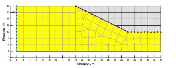
Figure 1. Problem configuration.
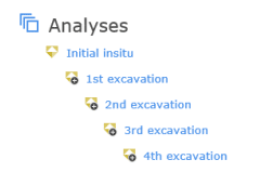
Figure 2. Analysis Tree for the Project.
Throughout the excavation process, and in the long term after the excavation has been completed, it is assumed that the water table on the left remains at the 16-m level. That is, the hydraulic boundary condition on the left remains the same at all times. The hydraulic properties used for this analysis are entirely arbitrary, selected purely for illustrative purposes. They can be viewed and inspected in the GeoStudio data file. Important to this type of analysis is the hydraulic boundary condition on the seepage face. The boundary condition must be a no-flow (Q=0) boundary condition with a potential seepage face.
The soil is treated simply as being Linear-Elastic, and the Poisson’s ratio is equal to 0.334 (1/3). The influence of Poisson’s ratio will be discussed below. The analysis here is a fully coupled SIGMA/W analysis.
As with all excavation analyses, the first step in the analysis process is to establish the in situ conditions. Recall that for a 2-D plane strain analysis,
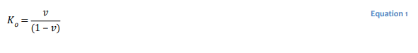
So, with equal to 1/3, 𝐾𝑜 is 0.5. The total unit weight of the soil has been set to 20 kN/m3 𝑣 , while the unit weight of water is 10 kN/m3. These values make it easy to spot check and discuss the results.
Results and Discussion
As is well known, when a saturated clayey soil is loaded, all or part of the load initially goes into the pore-water pressure, and then the pore-water pressure decreases as the soil consolidates. The reverse is true if the soil is unloaded. The unloading can cause the pore-water pressure to become negative and then increase with time as the soil swells. This response is evident in this excavation example.
Figure 3 shows the pore-water pressure contours one day after removal of the 2nd layer. Notice that the zero-pressure contour is well below the excavated surface; in fact, the negative pore-water pressure is more than -20 kPa below the base of the excavation.
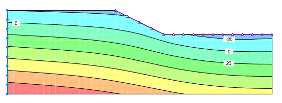
Figure 3. Pore-water pressure contours after removing the 2nd layer.
Figure 4 shows the pore-water pressure conditions one day after the 4th layer has been removed. Negative pore-water pressures still exist, but a seepage face has started to develop at the toe of the cut.
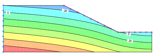
Figure 4. Pore-water pressure contours after removing the 4th layer.
Figure 5 shows the long term conditions about 2 months (60 days) after the excavation was completed. Now the pore-water pressure distribution represents a long-term steady-state seepage condition. There is a seepage face (zero pore-water pressure) at the cut toe and along the base of the excavation; the same as what one would get from a steady-state SEEP/W analysis.
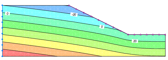
Figure 5. Pore-water pressure contours at the end on Day 80.
Another way to look at the results is to plot the pore-water pressure at a particular location for the duration of the analysis. Figure 6 shows the pore-water pressure with time at a location just below the final excavation level and slightly to the left of the final cut toe. Note how the pore-water pressure decreases each time a layer is removed and recovers with time.
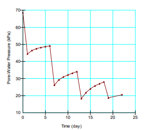
Figure 6. Pore-water pressure with time below and to the left of final cut toe.
Figure 7 shows the pore-water pressure changes at the final cut toe. Notice that the pore-water pressure goes to zero, since a seepage face has developed at that location.
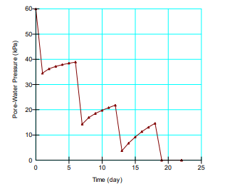
Figure 7. Pore-water pressure with time at final cut toe.
Special mention must be made of how to look at the excess pore-water pressures in a case like this. Figure 8 shows the excess pore-water pressure at the final cut toe. The graph indicates that the excess at the end is -60 kPa. The initial pore-water pressure before excavation started was +60 kPa. The amount of change is -60. So, the sum of the initial plus the change results in zero, which is the final pore-water pressure. In this case, the excess pore-water pressure is actually the change in pore-water pressure.
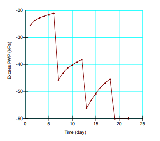
Figure 8. Excess pore-water pressures at the final cut toe.
The pore-water pressure response is influenced to some extent by the bulk modulus ( 𝐾𝑏), which is defined as,
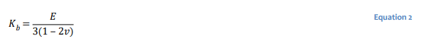
When Poisson’s ratio (𝑣) is one-third (1/3), 𝐾𝑏 is equal to 𝐸. That is, the bulk modulus is equal to the soil stiffness modulus 𝐸. Physically, this means that the stiffness of the soil plus the water is equivalent to the stiffness of the soil grain structure.
If we assume water is completely incompressible, 𝑣 is 0.5, and then 𝐾𝑏 goes to infinity.
Under field conditions, water likely always has some entrained air bubbles and, therefore, is never completely incompressible, and 𝐾𝑏 has some finite value even for saturated conditions.
This example was re-run with 𝑣 equal to 0.45 (data file and results are not included).
Figure 9 shows the difference in pore-water pressure response when 𝑣 is changed from the earlier 0.334 to 0.45. Generally, the pore-water pressures remain elevated longer all else being the same.
We recommend that you start with 𝑣 equal to one-third to establish a base case. Then you can try other 𝑣 values to determine what the effect is of considering different values.
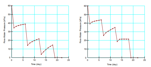
Figure 9. Pore-water pressure comparisons with ν = 0.334 and 0.450.
The most important parameter when it comes to real time calculations is the hydraulic conductivity. You should resolve what conductivity is appropriate and the effect it has on the solution before being too concerned about the bulk modulus.
Summary and Conclusions
This example demonstrates that SIGMA/W has all the capabilities and features to analyze the case of making an excavation below the water table, and to correctly compute the pore-water pressure response. Critical to this analysis is the ability to accommodate a moving hydraulic boundary condition, where the extent of a potential seepage face comes from the solution.