Introduction

In anticipation of the construction of a new airport in Bangkok, Thailand, full-scale test embankments were constructed on the soft clay at the site to study the effectiveness of prefabricated vertical drains (PVDs) for accelerating the consolidation and dissipation of the excess pore-water pressures resulting from fill placement. The results of the field tests have been studied and analyzed by two different research groups: one at the Asian Institute of Technology in Thailand, the other at the University of Wollongong in Australia. The findings are presented in two papers listed in the reference section below.

We have re-analyzed portions of this case history to demonstrate how GeoStudio can be used to model the effect of PVDs in the consolidation of soft soils. We have not attempted to replicate all aspects of the published information; rather our objective is only to provide sufficient information to show how GeoStudio users can do this type of geotechnical numerical modeling.

Numerical Simulation

The Bangkok Airport is situated in a wet area where there is about 10 m of soft clay under a 2 m surficial over-consolidated crust. Stiff clay, extending to a depth of 20 to 24 m, underlies the soft clay. For analysis purposes, the subsoil is divided into three layers (Figure 1) and the lower stiff clay is ignored.

Three test embankments were constructed, each with a different PVD spacing, but only the scenario with drain spacing of 1.5 m is discussed here. The PVD drains were installed to a depth of 12 m. The embankments were constructed to a height of 4.2 m with 3H:1V side slopes. The base areas were approximately 40 x 40 m. There were actually 1 m high berms around the base extending out 5 m, but this detail is not included in the illustrative GeoStudio analysis presented here.

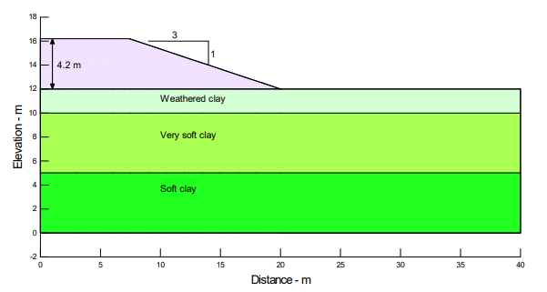
Figure 1. Configuration of Bangkok test embankment used in GeoStudio analysis.

A 1 m thick sand blanket was placed on the site as a construction working pad. The drains were installed from on top of the sand pad. The sand blanket was presumably also included to ensure that there would be no build-up of excess pore-water pressures at the base of the embankment and to drain away water being squeezed out of the clay.

The position of the drains in the two-dimensional analysis is shown in Figure 2. The horizontal spacing is 1.5 m except at the embankment toe where the spacing is 2 m (this was done purely for modeling convenience so that there is a drain at the embankment toe). Figure 2 also shows the layering used to simulate the sequential fill placement.

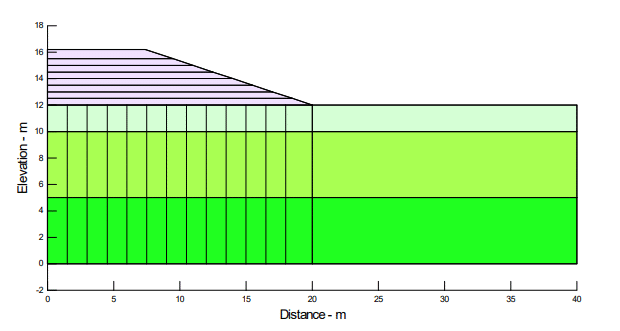
Figure 2. Position of the vertical drains and layers used for sequential fill placement.

The sand blanket is not included in the model as a separate material. The effect of the sand can be modeled by specifying a zero-pressure boundary condition along the ground surface. The physical implication is that there will be no build-up of positive pore-water pressures at the ground surface. Any water arriving at the ground surface will have the opportunity to disappear through the sand somehow; the boundary condition simulates this effect. This is much simpler than trying to include the sand blanket in the model, but achieves the same objective.

The Modified Cam-Clay constitutive relationship is used here for the soft clay. The parameters used can be viewed in the GeoStudio data files. The clay is essentially normal to slightly over-consolidated. It appears that the degree of over-consolidation varies somewhat with depth. For the illustrative analysis here, the clay is treated as having an over-consolidation ratio (OCR) of 1.5. Also, the Lambda and Kappa values were taken to be the same for the very soft and the lower soft clay. This gives settlements closer to what was measured.

The weathered surficial clay is over-consolidated and, consequently, it is acceptable to treat this layer as behaving in a linear-elastic manner. Using a linear-elastic constitutive relationship also helps with maintaining numerical convergence near the ground surface where the stresses approach zero.

The sand fill is also treated as a soft linear-elastic material and the soil parameters are viewed as being total-stress parameters. This avoids having to deal with pore-water pressures in the fill. These simplifying assumptions are acceptable because we are primarily interested in using the fill as a means to apply the load. The actual stress-strain response of the sand is not of significant importance.

The most critical parameter in an analysis like this is the hydraulic conductivity (coefficient of permeability). By the very nature of the deposition process, the conductivity can vary significantly. In addition, the stratification tends to make the conductivity somewhat higher in the horizontal direction than in the vertical direction. Furthermore, the insertion of the drains disturbs the soil around the drain and alters the conductivity. The disturbed zone is often called a smear zone.

Drains are installed in some kind of pattern and spacing and flow to the drains is two-dimensional in plan view. Analyses, however, are generally more conveniently carried out in a 2D cross-section.

Indraratna and Redana (2000) have done extensive studies on how to adjust conductivities for a 2D plane-strain analysis, how to assess the smear zone thickness and conductivity, and how to model the size of the drain itself. The details are in the paper reference cited at the end. A brief summary is presented here to show how these effects can be accounted for in a GeoStudio analysis.

The flow is predominately horizontal to the drains and, consequently, most of the discussion centers around the horizontal conductivity (𝐾𝑥 ). In GeoStudio, the vertical conductivity (𝐾𝑣 ) can be a ratio of the horizontal conductivity, but this is not all that important since there is very little or no vertical
flow.

where 𝑎 is the thickness of the PVD drain and 𝑏 is the width. So, for a typical drain that is 4 mm thick and 100 mm wide, the 2D model thickness can be 66 mm or say 0.06 m. In GeoStudio, the drain can be represented with an interface element that is 0.06 m thick, for example.

The simplest form of converting from an axisymmetric to plane-strain conductivity is:

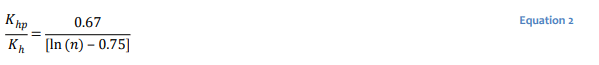
where 𝑛 is the ratio of the drain spacing (𝐷) to the equivalent drain thickness (𝑑𝑤). If the drain  spacing is 1.5 m and the equivalent drain thickness is 0.06, then 𝑛 is 25. The plane-strain conductivity then is about 27 percent of the corresponding axisymmetric horizontal conductivity. This is in the absence of any well resistance and any effect of a smear zone. As an easy figure to remember, the plane-strain conductivity is about a quarter of the corresponding axisymmetric conductivity.

Indraratna and Redana (2000) suggest that the radius of a smear zone around a drain will typically be five (5) times the equivalent radius of the mandrel. For a mandrel that is 45 mm thick and 125 mm wide, the equivalent radius is about 55 mm. The radius of the smear zone then is 270 mm (0.27 m). For a 2D analysis, the smear zone thickness would then be 0.54 m.

Indraratna and Redana (2000) have presented an equation to estimate the conductivity of the smear zone which involves various dimensional ratios and conductivity ratios. We will not go into all the details here, as they are available in the Indraratna and Redana (2000) paper for those interested. As a broad rule, the horizontal smear zone conductivity is about 10% of the horizontal plane-strain conductivity. For the cases presented by Indraratna and Redana (2000), the ratio varies between 8-16%. Stated another way, the disturbance resulting from the insertion of the drain reduces the conductivity by about an order of magnitude in the smear zone.

With flow across a layered system, the less permeable layer can quickly dominate the head loss and, in turn, govern the flow behavior. Consider the simple layered system in Figure 3, where each segment is 1 m long. A total head (H) of 10 m is applied on the left end and a total head of 1 m on the right end. The conductivity of the right segment is 10 times less than on the left. The head loss distribution across the system is as shown in Figure 4. Note that most of the head loss occurs in the less conductive material and the gradient is much higher in the less conductive material. In other words, the less conductive material on the right essentially governs the flow.

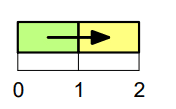
Figure 3. Flow in a layered system.

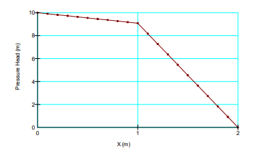
Figure 4. Head loss distribution in a layered system.

For a layered system like this, we can compute an equivalent conductivity as follows:

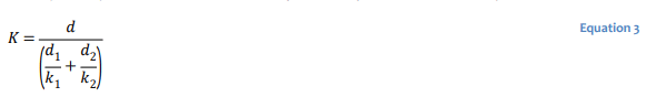
Say 𝑑1 is 1 m, 𝑑2 is 1 m, 𝑘1 is 10 m/sec and 𝑘2 is 1 m/sec. The blended equivalent 𝐾 then is 1.818 m/sec. We can use this information to represent the conductivity of the native clay together with the smear zone rather than create separate geometric regions for the two different zones. This makes the numerical modeling easier.

The implication for our analysis is that the smear zone around the drain dominates the dissipation of the excess pore-water pressures and, in turn, the rate of consolidation.

Indraratna and Redana (2000) presented a table of conductivities used in their analyses. For a 1.5 m drain spacing, the conductivities are as in Table 1, where the conductivities have been converted to m/day. The blended 𝐾 is computed based on drain spacing of 1.5 m (radius = 0.75 m) and a smear zone thickness of 0.54 m (radius = 0.27 m). For discussion and mental interpretation purposes, it is worth noting that the soft clay at depth has a conductivity of about one order of magnitude less than the upper weathered clay.

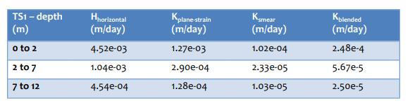
Table 1. Conductivities used in the analysis presented by Indraratna and Redana (2000) converted to m/day.

The conductivity of soft soils can change significantly as the soil compresses and the void ratio decreases. GeoStudio has a mechanism whereby the conductivity can be adjusted as the effective stress increases in response to the dissipation of the excess pore-water pressure. This is an indirect way of adjusting the conductivity resulting from a decrease in void ratio.

One way to define data for such an adjustment in conductivity is from the results of an odometer test. The conductivity can be computed for each load increment in an odometer test as follows. The change in effective stress and void ratio measured over each load increment can be used to determine the coefficient of compressibility:

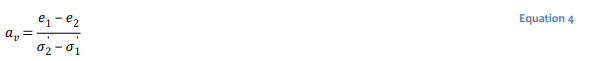
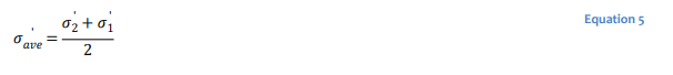
and the average vertical effective stress:

For each load increment, a void ratio versus time plot is available which can be used to determine the coefficient of consolidation (𝐶𝑣). Once these values are known the conductivity can be computed from:

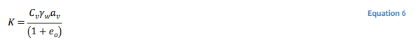
In this way, 𝐾 can be determined for the average vertical effective stress for each load increment. This data can be entered in GeoStudio to create a curve like the one shown in Figure 5.

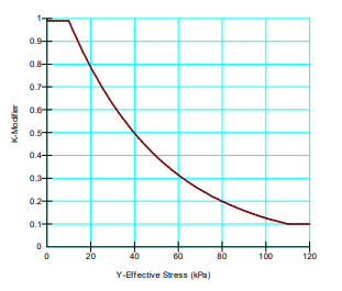
Figure 5. An illustrative conductivity (𝐾) modifier function.

This graph, in essence, says that conductivity obtained from the specified hydraulic conductivity function will reduce as the effective stress increases. For this illustrative graph, the conductivity would diminish one order of magnitude with a change in vertical stress from 10 kPa to 100 kPa. A modifier value of 1 should represent the average effective stress state at which the conductivity was measured and defined in GeoStudio.

The curves used in the analyses presented here can be viewed in the data files. The specified conductivity is assumed to be at the effective stress close to the top of the corresponding layer. This type of data is not available for the Bangkok site, but such a modifier function is included in the analysis here nonetheless to illustrate the use of this feature in GeoStudio. The curves are purely estimates for illustrative purposes.

From a modeling perspective, it is best in a case like this to start with analyzing just one cell. It makes the modeling process much more manageable while the key issues are being resolved. So, to begin with, let us look at a single cell.

Figure 6 shows a single cell with a 1.5 m drain spacing. The drain is in the middle of the cell.

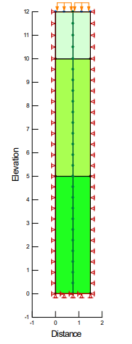
Figure 6. One cell with a boundary condition to represent the effect of the drain.

In this case, we will treat the drain as a “perfect” drain, meaning that there is no head loss in the drain or no well resistance. We can model this condition with a specified boundary condition. Making the boundary condition a total head equal to 12 m (H = 12) says that the pressure distribution will be perfectly hydrostatic at all times.

Recall that when we specify a head or pressure at a node, the finite element analysis will compute a flux (Q) at that node. So specifying a head at the drain means flow comes out of the system at these nodes. This is not what happens physically, but numerically it is equivalent to water flowing out of the top of the drain where there is no head loss due to the flow.

The pore-water pressure across the top is set to zero to represent the water table at the ground surface. We can assign the soil the blended conductivity based on the reasoning presented above.

The loading from the embankment can be applied with a pressure type boundary condition (Figure 7). There are long periods with no increase in the loading while the pore-water pressure is allowed to dissipate. Also, the time can run past the end of the graph at 300 days. It simply means there is no more loading, but the pore-water pressure can continue to dissipate. The analysis is carried out up to 400 days.

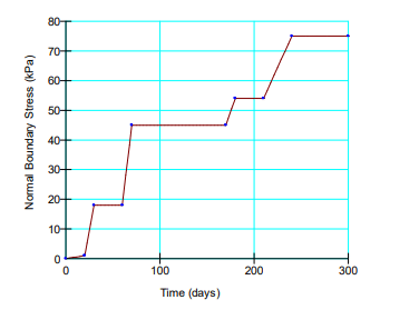
Figure 7. Applied pressure to represent the embankment fill placement.

The computed surface settlement is shown in Figure 8. The total settlement is about 0.85 m. The field measured settlement after 400 days of consolidation was around 1 m. This suggests that the one-cell model is a reasonable representation of the actual field conditions.

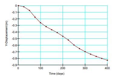
Figure 8. Surface settlement with 1.5 m drain spacing.

One other observation of significance is that the largest part of the compression occurred in the very soft clay (Figure 9). About 90% of the total 0.85 m of settlement is in the very soft clay. Also very little compression occurs on the surficial over-consolidated crust.

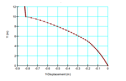
Figure 9. Settlement profile at the end of 400 days.

This type of information is valuable to assess the material properties selected for each of the layers. At this stage, adjustments could be made if deemed necessary before proceeding to a full scale 2D analysis.

The excess pore-water pressure at the mid-way point between two drains (edge of model for one-cell case) is shown in Figure 10. These pore-water pressures are at the contact between the very soft clay and the underlying slightly more competent clay. These pore-water pressures are higher than what was reported by Indraratna and Redana (2000). The reason for the difference is not clear. Let’s leave this for now and re-examine this later again after further analysis.

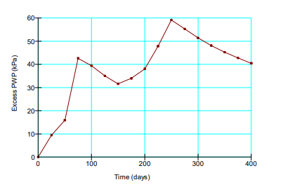
Figure 10. Excess pore-water pressures at the mid-way point between two drains at the contact between the very soft clay and the underlying slightly more competent clay (El 5 m).

The drain itself can actually be modeled with what are known as interface elements. The drain is included with special finite elements with their own properties (Figure 11). The drain in this case is sometimes referred to as a well.

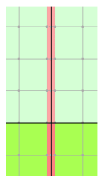
Figure 11. Interface elements represent the drain or well.

For the analysis here, the drain (interface) is given the same mechanical properties as the surrounding soil. This is to say that the mechanical stiffness of the drain has no effect on the behavior. The well resistance can be modeled with an equivalent hydraulic conductivity. A very high 𝐾 value means little or no resistance and a low 𝐾 would mean some well resistance.

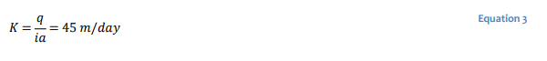
An approximate 𝐾 can be estimated from a known discharge capacity for a particular drain design and consideration of Darcy’s law. Let’s say the discharge capacity is 100 m3/year – this is about 0.275 m3/day. Also, let’s assume the head loss in the 12 m long drain is 1.2 m. In our model, the drain thickness is 0.06 m. With a unit thickness, the drain cross-sectional area is 0.06 m2. The equivalent 𝐾 is then:

Results and Discussion

The following graph (Figure 12) shows the excess head in the well on Day 250 when the pore-water pressures are generally the highest. The excess head at the base of the well is only about 0.5 m.

Also, the computed surface settlement is more or less the same as the case of a perfect drain. This indicates that at a K of 1 m/day for the drain, the well resistance is not a factor.

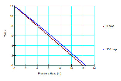
Figure 12. Excess pressure head distribution in the well.

If we reduce the well K by an order of magnitude to 0.1 m/day, the excess head distribution is as shown in Figure 13. Now there is about 3.5 m of excess head at the base of the well and the total settlement is approximately 0.67 m as opposed to the 0.85 m with a perfect drain. In other words, the well resistance is now affecting the pore-water pressure dissipation and settlement.

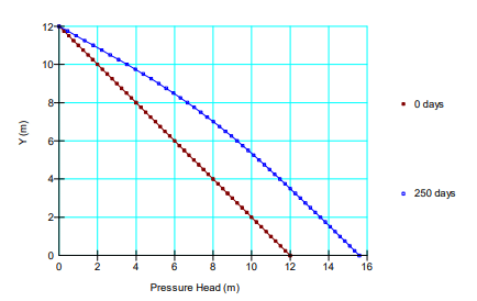
Figure 13. Excess pressure head distribution in the well with a reduced conductivity.

It is difficult to exactly quantify the well resistance, particularly if the drains become damaged or partially clogged. The procedure described here at least makes it possible to investigate the effect of resistance to flow in the drains.

Another important observation is that if we make the assumption that there is no well resistance, then we can simulate the drains with a boundary condition. This greatly simplifies the modeling, especially for 2D field cases.

If we now use the same properties in a 2D field model as were used in the one-cell analyses, the surface settlement profile is as shown in Figure 14. The total computed settlement under the centerline of the embankment is 1.2 m. This is somewhat higher than the 0.85 m computed for the one-cell analysis. The exact reason for the difference is not entirely clear. One difference between the analyses is the loading. Simulating the actual fill placement results in a different loading pattern than used for the one-cell analysis. There are of course some two-dimensional effects which can also have an effect. The 2D and one-cell results are close enough that a good picture of the settlement can be obtained from a one-cell analysis. The 1.2 m of settlement is reasonably close to the value measured in the field.

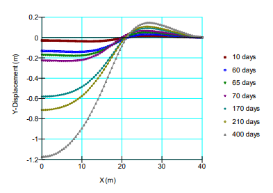
Figure 14. Ground surface settlement profiles in 2D field model.

Figure 15 shows the deformation at the end of 400 days as a deformed mesh at a true 1:1 scale (no exaggeration). This provides a picture of the overall settlements.

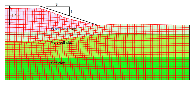
Figure 15. Settlements presented as a deformed mesh.

Summary and Conclusions

These analyses show that GeoStudio has all of the features to model the effect of prefabricated vertical drains installed to aid in the dissipation of excess pore-water pressures in soft soil arising from surface loading. The results presented here are somewhat different than that reported by others. Our objective here is not necessarily to replicate exactly what others have done. The objective is to demonstrate that GeoStudio has the capability to do this type of analysis and the trends in the results are sufficient to confirm that this is the case. More could likely be done to match the published information but the effort is not warranted in light of these objectives.

The results ultimately come down to the one overriding controlling parameter which is the hydraulic conductivity of the clay. As is well known, the conductivity of natural marine deposits can vary significantly, often within an order of magnitude. In addition, in cases like this, we have the disturbance of the clay and the effect this has on the conductivity due to the insertion of the drains. So the accuracy of predicting the rate of the settlement is directly related to the confidence with which the conductivity can be defined and to what degree the drains will become clogged and damaged. Careful consideration needs to be given to the results in the context of this field reality.

There are several modeling lessons in this demonstration. Much of the behavior can be studied with a simple one-cell model. Any study like this should at least start with a one-cell analysis to resolve most of the modeling issues before proceeding to a 2D field analysis. The effect of the drains can be modeled with boundary conditions. It is not necessarily a requirement that the actual physical drains are included in a complex 2D analysis – it can unnecessarily over-complicate the model. As always, the best lesson is to start simple and gradually move to the more complex in stages.

References

Bergado, D.T., Balasubramian, A.S., Fannin, R.J. and Holtz, R.D. (2002). Prefabricated vertical drains (PVS’s) in soft Bangkok clay: a case study of the new Bangkok International Airport project, Canadian Geotechnical Journal, Vol. 39, pp. 304-315.

Indraratna, B. and Redana, I.W. (2000) Numerical modeling of the vertical drains with smear and well resistance installed in soft clay, Canadian Geotechnical Journal, Vol. 37, pp. 132-145