An Introduction to Resource Estimation using Leapfrog Edge

Join us for an introduction to learn the fundamental tools necessary to get you going, including numeric data analysis, defining a domain, variography, producing robust estimates, validating and reporting, the Leapfrog way.

Overview

Video Transcript

[00:00:00.900]<v Steve>Thank you for joining me today.</v>

[00:00:02.620]My name’s Steve Law.

[00:00:03.777]I’m a senior geologist with Seequent,

[00:00:06.500]based in the Perth office.

[00:00:09.260]My background is in resource geology

[00:00:11.270]and mining geology.

[00:00:12.680]And today we’ll take you through

[00:00:15.710]the new Leapfrog Edge resource module.

[00:00:19.740]Before we go into the software demonstration,

[00:00:22.310]I’d just like to present a brief presentation

[00:00:26.700]talking about when Edge can benefit you

[00:00:30.999]and how it fits into

[00:00:32.550]a Seequent workflows.

[00:00:36.620]Seequent works across all different sectors.

[00:00:40.020]Today we’ll be concentrating on the mining

[00:00:42.190]and minerals sector,

[00:00:43.460]which basically uses Leapfrog Geo.

[00:00:46.070]We also have Leapfrog Energy for the energy market,

[00:00:49.470]and recently Edge was introduced there as an option as well.

[00:00:53.160]And we have in the civil and environmental sector,

[00:00:56.350]we have Leapfrog works at this stage.

[00:00:58.700]Edge cannot be used with Leapfrog works.

[00:01:01.660]Most of you are familiar with Leapfrog Geo

[00:01:04.430]that Leapfrog Geo and now Edge

[00:01:06.620]are part of a whole ecosystem

[00:01:09.560]for Seequent.

[00:01:12.120]The basic building blocks are Leapfrog Geo,

[00:01:15.040]Leapfrog Works and Leapfrog Energy

[00:01:17.030]and Leapfrog Edge is not a standalone option.

[00:01:19.960]It is a module within Leapfrog Geo and Leapfrog Energy,

[00:01:24.907]and is the main engine used by geologists

[00:01:28.570]and models to produce the 3D models.

[00:01:32.060]Sitting above that now we have Seequent Central.

[00:01:37.160]That is a system that helps organize our projects

[00:01:40.274]and is a fantastic tool for people to share

[00:01:43.650]the same projects across different parts

[00:01:46.380]of their organization at the same time.

[00:01:48.840]And it’s also useful for collaborating

[00:01:51.306]between especially different locations.

[00:01:54.990]People can have access to just looking at the model

[00:01:57.717]or they can have access to working with the model.

[00:02:01.870]Sitting above that again is Leapfrog View.

[00:02:05.120]Some of you may be familiar with Leapfrog Viewer,

[00:02:07.830]which has been available for quite some time,

[00:02:10.250]but that one requires you to download

[00:02:12.400]the software onto your desktop.

[00:02:14.420]Leapfrog View is a browser based version

[00:02:16.970]of this and enables you to share your projects

[00:02:20.190]in the 3D environment,

[00:02:22.740]simply by people having a look at a browser

[00:02:25.830]to still secure linkages, to share,

[00:02:28.430]so that only the people you wish to see

[00:02:30.240]the information can do so,

[00:02:32.140]but it also has some great tools for sharing

[00:02:35.790]and collaboration.

[00:02:38.870]We’re going to focus today on Leapfrog Edge,

[00:02:41.690]but I will be using Central as the platform

[00:02:44.530]to access the project.

[00:02:45.830]So you’ll have an idea of how it looks

[00:02:47.567]and towards the end of the webinar,

[00:02:49.710]I will just give a brief mention

[00:02:51.960]on how you can restructure

[00:02:53.800]the way you manage your projects

[00:02:55.530]if you’re using Edge and Geo at the same time,

[00:02:58.280]and you have Central available.

[00:03:03.290]Main reasons why we might want to consider using Edge,

[00:03:06.820]it has all the same capabilities or efficiencies

[00:03:10.650]and advantages that Leapfrog has.

[00:03:13.420]Some of these include time efficiency.

[00:03:17.800]It is not a difficult program to learn to use.

[00:03:20.540]As you’ll see today after the demonstration,

[00:03:22.920]it has a quite intuitive interface and workflow.

[00:03:26.860]And as always the initial models

[00:03:28.870]can take time to build up

[00:03:30.500]and having to go through all this standard resource

[00:03:33.510]estimation steps that we need to follow.

[00:03:35.766]But the time efficiency really comes in

[00:03:38.670]after the original model.

[00:03:40.100]And when you’re working with updates,

[00:03:41.970]because everything is on automatically linked to your data,

[00:03:45.890]to your geological model,

[00:03:47.450]then the associated block models will update

[00:03:50.910]as well as all the validation reports

[00:03:53.320]and subsequent resource reporting tools.

[00:03:56.943]Integration is a major importance.

[00:04:00.790]So rather than having to jump in

[00:04:02.670]and out of various softwares

[00:04:04.560]to do the different aspects

[00:04:05.950]of a resource estimation,

[00:04:07.740]you can, it’s all done in the one spot.

[00:04:10.350]You don’t have to worry about conventions

[00:04:13.006]from when you transfer,

[00:04:14.580]say a very grant from one package to another,

[00:04:17.140]it’s all in built and ready to go.

[00:04:20.310]And then my significant benefit is the visualization.

[00:04:24.670]We’ve carried through the Leapfrog Geo visualization tools

[00:04:28.840]and benefits to Edge.

[00:04:30.743]So that at all parts of the estimation process,

[00:04:34.360]you’re able to see what’s happening with your data

[00:04:37.650]in the 3D scene and vice versa

[00:04:40.040]as you fill in different forms and table forgets.

[00:04:43.070]We still went through the standard process

[00:04:45.560]that we use for any resource system motion.

[00:04:48.020]So with the underlying geology and the geology model

[00:04:51.870]is extremely important as always.

[00:04:54.150]And we can look at our compositing

[00:04:56.380]our exploratory data analysis,

[00:04:59.360]very all graphy, the XO estimation parameters,

[00:05:02.480]and then that vengeful validation,

[00:05:05.010]but having rather than having to work

[00:05:07.030]in a continuously linear workflow.

[00:05:09.450]And sometimes we do get as resource geologists lost

[00:05:12.950]in the numbers.

[00:05:14.200]We were always with Leapfrog Edge in Geo together,

[00:05:17.660]keeping the geology at the forefront

[00:05:19.920]as we worked through the process.

[00:05:21.760]So we can easily step backwards and forwards

[00:05:24.400]between the model and what we’re trying

[00:05:26.350]to achieve with the estimate.

[00:05:28.460]And this is done in a very visual way,

[00:05:31.910]which helps us work through the whole process.

[00:05:35.820]Today in the demonstration, which we’ll start in a moment,

[00:05:38.910]we are going to at least briefly cover all

[00:05:41.410]of these different steps.

[00:05:42.243]So I’m going to try and show you the entire workflow

[00:05:44.950]from beginning to end.

[00:05:47.377]I won’t be going into some of the finer details

[00:05:49.920]of how you need to do this.

[00:05:51.967]And at the end of the presentation,

[00:05:54.970]I’ll show you how to be able to have access,

[00:05:58.690]to learning some more about how Edge works

[00:06:02.338]ways in which people are currently using Edge.

[00:06:05.020]So it took about three years of development

[00:06:08.490]and it was first released in 20, late 2017.

[00:06:12.090]Since that time it’s been undergoing continuous improvement

[00:06:15.733]and we’ve had a few people,

[00:06:18.290]quite a few people start to use it now.

[00:06:20.760]Some of the key areas

[00:06:21.880]it’s being used in early evaluation

[00:06:25.750]or during resource in fields, really.

[00:06:28.680]So it’s great.

[00:06:30.210]Even with sparse data,

[00:06:31.745]being able to generate results

[00:06:34.090]and at least give you an idea

[00:06:36.565]of what your resource may be in the future

[00:06:40.050]with resource infill drilling,

[00:06:42.410]we’ve had some clients use it

[00:06:43.730]as they actually do the drilling.

[00:06:46.140]They input the results as they come in

[00:06:49.250]and they get an impression

[00:06:50.290]of how the block model may change.

[00:06:52.670]And then they can modify their drilling program a little.

[00:06:55.550]If they find that one area of the resource,

[00:06:58.290]isn’t really changing,

[00:06:59.380]no matter how many holes you put into it,

[00:07:01.360]but it might unexpectedly point to some other open areas.

[00:07:05.170]So rather than having to wait a few months

[00:07:06.780]after you’ve done all the data input

[00:07:08.890]and the geological modeling,

[00:07:10.540]you can get some,

[00:07:11.373]at least early ideas during the drilling.

[00:07:14.970]Another area where people are using it in is Grade Control.

[00:07:18.720]So this is where the dynamic factor of it is great

[00:07:22.700]because it’s already linked to the data base

[00:07:24.720]and the geological model,

[00:07:26.970]as soon as the new data goes in,

[00:07:28.950]the block model will update and you’ll get

[00:07:31.970]instant reports on how things are changing.

[00:07:35.710]And then it is being used

[00:07:38.010]for standard resource estimation and reportable resources.

[00:07:45.100]More of it it’s been used in other areas of the world

[00:07:49.860]where we’ve got quite a few

[00:07:51.360]in our 43101 reports now started

[00:07:53.850]to use Edge as a fundamental software

[00:07:57.000]that they’re doing their reporting on.

[00:08:03.170]So I will now go into the software presentation.

[00:08:10.720]So what we’re looking at here is a screenshot

[00:08:13.970]of what Central looks like.

[00:08:16.530]So I have just downloaded from a Central server,

[00:08:21.420]the model that we’re going to be working with today.

[00:08:24.630]What Central does is it serves you

[00:08:27.130]basically maintains coffee of all projects.

[00:08:30.640]So since the very first time

[00:08:31.940]that I started working on this project

[00:08:34.040]and working on either a geological model section of it

[00:08:38.560]or the estimation it’s storing the results,

[00:08:41.290]so that at any time we can go backwards

[00:08:43.560]and see what happens,

[00:08:44.650]say six months or a year ago,

[00:08:47.420]when I want this, the most recent project,

[00:08:50.320]the one at the top here,

[00:08:51.610]I can download that,

[00:08:52.956]which I’ve already done that downloads

[00:08:55.440]a copy directly to your computer.

[00:08:57.700]So this is how we can have multiple users using

[00:09:00.510]the same project,

[00:09:01.400]whereas standardly Leapfrog Geo,

[00:09:04.120]that’s not possible.

[00:09:06.180]And then people can work on different aspects,

[00:09:08.450]say the geology model,

[00:09:09.730]the estimation, or even the fault modeling.

[00:09:12.440]And then it does take some management

[00:09:14.330]on making sure all those things get put back together again.

[00:09:17.820]So I’m going to open up this project here.

[00:09:39.980]We’re going to be working with a fairly simple model today,

[00:09:43.560]just so that we can get the key aspects

[00:09:50.290]of Edge across to you.

[00:09:53.750]So what we’re looking at is

[00:09:57.900]a simple set of drew halls.

[00:10:00.300]We’ve got asset data,

[00:10:01.550]we’ve got copper data in this instance.

[00:10:08.530]Simple geological bottle has been made up now, ideally itch.

[00:10:13.990]The idea is that you do have a geological model.

[00:10:17.892]It was in the same project or accessible via Central,

[00:10:23.240]but you can use Edge directly on imported meshes.

[00:10:27.280]So if you’ve got a wire frame

[00:10:29.810]that you’ve brought in from another software,

[00:10:32.040]so the domaining has been done somewhere else,

[00:10:34.710]you can still import that into the meshes folder

[00:10:37.070]of Leapfrog and run the estimation, purely on those.

[00:10:41.720]As long as you’ve got the drill hole database

[00:10:43.630]that you need to use and some kind of solid volume,

[00:10:47.630]then you’ll be able to run an Edge estimate.

[00:10:52.770]We have various tools for understanding

[00:10:55.950]our data prior to starting the estimation.

[00:10:59.270]So running an exploratory data analysis,

[00:11:03.560]so we can do this at different levels.

[00:11:05.650]We can do it at the database level.

[00:11:09.618]So for instance,

[00:11:10.451]if I want to know a little bit about my copper data up here,

[00:11:14.660]I right click and I can look at my statistics.

[00:11:18.160]And because we’re just looking at a single element within

[00:11:24.960]a table,

[00:11:27.950]it just serves as a histogram.

[00:11:30.490]These can be detached.

[00:11:33.267]And as long as I have that information visible in the scene,

[00:11:41.330]we’ll see that if I highlight part of the histogram,

[00:11:43.750]for instance,

[00:11:44.583]I would like to know where these higher values are,

[00:11:46.760]then that data is interactive with the 3D scene.

[00:11:50.540]So any part of the histogram that we highlight

[00:11:53.179]the corresponding intervals will show up in the 3D scene.

[00:11:57.540]So that’s one way of understanding

[00:11:59.300]that this spatial distribution of our data.

[00:12:04.603]This is available through all of our graphs.

[00:12:09.082]We have other ways of looking at our data.

[00:12:17.230]In terms of just visualizing the information

[00:12:20.270]as well as fixed radius,

[00:12:22.210]so we’ve basically just looking at a solid cylinder.

[00:12:25.690]If we’ve turned on this little pink button here,

[00:12:27.860]we can go back to just traces or we can make

[00:12:31.010]the line more solid

[00:12:33.950]and you can change the size of that.

[00:12:52.350]The other alternative is we can use

[00:12:56.440]the other elements that are available within our table.

[00:12:58.890]So in this instance, we’ve got gold as well.

[00:13:01.290]We can display by copper colors,

[00:13:04.860]but by the radius of the gold content,

[00:13:09.553]as well as that, we also have graph capability.

[00:13:13.990]So underneath your survey table,

[00:13:16.640]on the left-hand side,

[00:13:18.130]we have drew whole graphs.

[00:13:19.980]If we drag them in,

[00:13:26.276]you can see here that we can display any of that.

[00:13:28.870]We can look at gold,

[00:13:30.660]we can scale it so that the bars are so up.

[00:13:33.960]I’ll just say that in 3D there,

[00:13:37.710]and we can offset.

[00:13:38.740]So if we have put a cylinder on,

[00:13:40.720]we can move it a little bit away from the drill hall traces.

[00:13:44.940]So into…

[00:13:52.155](sighs)

[00:14:06.475]We have a look in section,

[00:14:12.710]you can see that we’ve got the graphs on the side,

[00:14:16.950]copper despite all size color,

[00:14:18.660]and the disk or side done by a scale.

[00:14:25.470]If we’re using merge tables

[00:14:26.760]where we may have merged together lithology

[00:14:29.610]with essay data.

[00:14:31.000]So in this case,

[00:14:31.870]I’ve got some lithology and essay data grouped together.

[00:14:34.980]Well, then this will give us access

[00:14:36.930]to some other graphing features.

[00:14:40.170]One of the most useful ones is the box plot.

[00:14:44.150]So we tell them we need to have a numeric column.

[00:14:46.580]We need a categorical column in this case, it’s rock.

[00:14:49.890]And when we can see a box plot,

[00:14:52.790]sewing the information.

[00:14:54.220]So this is a great way of looking at new data sets.

[00:14:57.260]If you’ve got a lot of codes you’re unfamiliar with,

[00:14:59.840]we might quickly be able to determine

[00:15:01.470]which of the most important codes

[00:15:03.085]for relating the essays back to the geology.

[00:15:07.839]If you want to just get the numeric information

[00:15:10.640]out of there in the statistics,

[00:15:13.040]there is a table of statistics and you can see

[00:15:16.513]that the means, et cetera,

[00:15:18.760]for all that data and anything

[00:15:20.750]that’s available within those tables.

[00:15:27.840]We’ll now move more into Edge.

[00:15:29.700]So the way to know whether you have access to Edge

[00:15:38.540]is whether or not you have this estimation folder

[00:15:41.710]present in your project.

[00:15:44.560]If you just have Leapfrog Geo on your license,

[00:15:46.920]then that estimation folder will not show,

[00:15:49.430]but once you have Edge activated, it will.

[00:15:52.330]And everything that we need to do to set up Edge parameters

[00:15:55.610]is done inside this estimation folder.

[00:15:58.740]All the results though are viewed by the block models.

[00:16:02.390]If someone has used Edge and created an eye block model,

[00:16:06.240]you do not need an Edge’s license

[00:16:07.980]to view the results of that.

[00:16:09.350]So next time you open that project,

[00:16:11.613]even if Edge isn’t available,

[00:16:14.340]you will still be able to look at the plot model results.

[00:16:17.410]And generally in that instance,

[00:16:19.250]the estimation fold will have a little restricted

[00:16:22.040]sign standing next to it.

[00:16:25.540]The whole premise of using Edge is working

[00:16:28.370]on a domain by domain basis.

[00:16:33.780]So where you build up your Edges,

[00:16:37.150]you right-click, and you basically create

[00:16:39.140]a new domain estimation.

[00:16:44.420]From there,

[00:16:45.253]you can pick out your domain.

[00:16:48.070]So this shows here that it can be accessed

[00:16:51.003]from anything that’s within the meshes folder.

[00:16:54.720]So if you’ve got a WiFi from elsewhere,

[00:16:57.900]just put it in here and you can access it in this instance,

[00:17:01.720]the blue meshes mean that these are being accessed

[00:17:04.140]from a different project within Leapfrog’s Seequent Central.

[00:17:08.800]Also any volumes within your geological models,

[00:17:12.580]so in this case, it’s the output volumes,

[00:17:15.370]but we can also use solids like intrusions

[00:17:18.880]or veins from within the surface chronology as well.

[00:17:23.106]You can also access any of the great shells

[00:17:25.710]we may have generated from an numeric model.

[00:17:28.710]So all of these things available to choose from.

[00:17:34.180]I’m just going to pick out this early thyroid.

[00:17:45.410]Again, in terms of the essay data,

[00:17:48.270]it’s sourcing anything

[00:17:49.670]that’s within your geological database.

[00:17:51.810]So you’ve got your raw data.

[00:17:53.910]You’ve got any data

[00:17:54.850]that you’ve made a composite file from

[00:17:56.950]at the database level, merge tables

[00:18:00.471]and we can also use point data within a estimate as well.

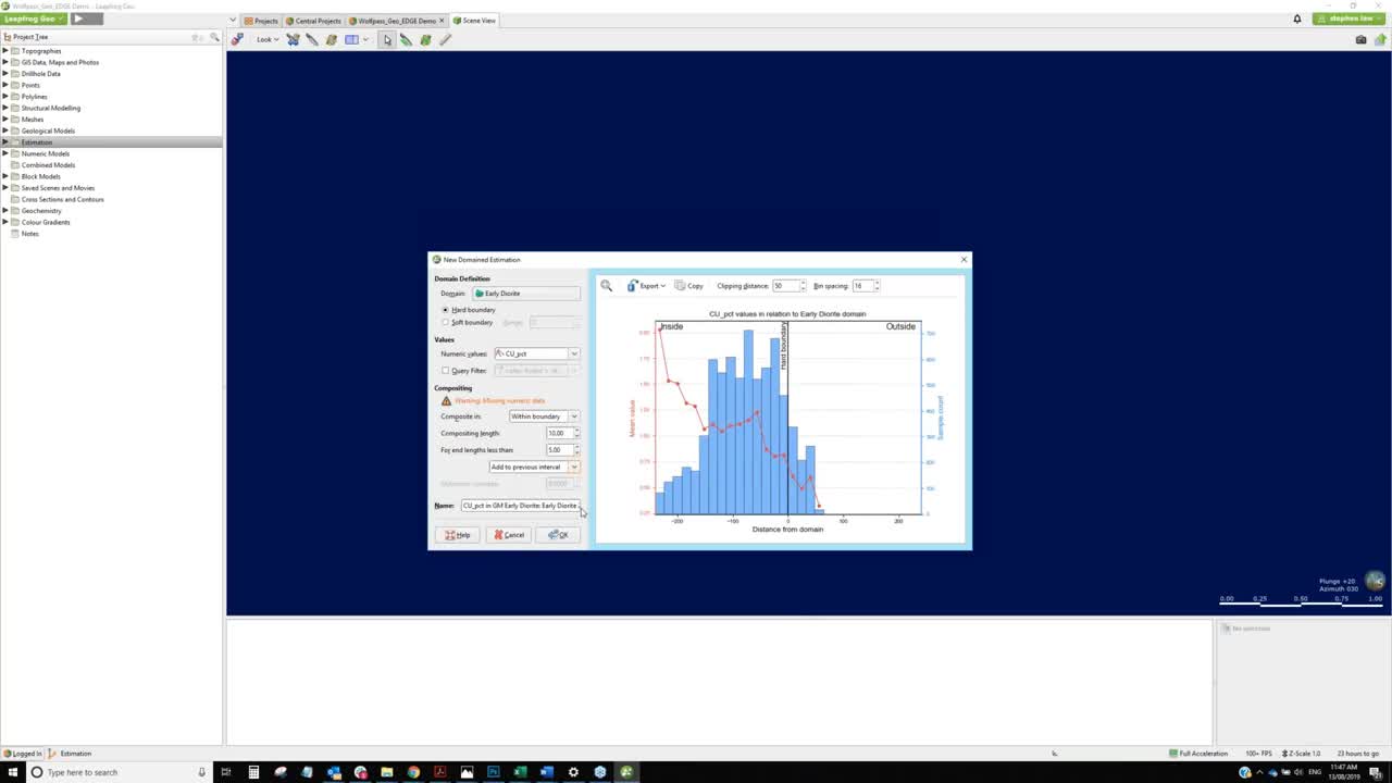
[00:18:05.320]So in this instance,

[00:18:06.890]I’m not going to composite at this level.

[00:18:10.400]I’m going to do it later on.

[00:18:12.110]We have two options for compositing.

[00:18:14.080]You can either do the compositing prior

[00:18:16.420]to running the estimation.

[00:18:18.130]So that’s setting it up under the database,

[00:18:20.420]under the composites folder

[00:18:22.070]and running our standard numeric composite tools.

[00:18:26.808]Or we can compensate on the fly,

[00:18:28.570]which is what I’m going to show you today.

[00:18:31.430]I’ve used copper percent

[00:18:33.170]and this is where we can choose to use compositing here.

[00:18:36.870]At this stage,

[00:18:37.890]it is usually always within a boundary.

[00:18:39.829]So it is going to honor the boundaries

[00:18:42.030]of the particular domain that you’re working with.

[00:18:46.500]And then we have our standard compositing tools

[00:18:50.860]for determining what we’re going to do

[00:18:53.420]with the little pieces at the end.

[00:18:55.510]So we can either discard add to the previous interval

[00:18:58.990]at the end of the whole

[00:19:00.403]or distribute it across equally across the whole domain.

[00:19:06.510]You can try different ways

[00:19:07.790]to see how sensitive your data is to compositing.

[00:19:12.420]We always end up with a default name at this stage,

[00:19:14.750]and this becomes the name for the estimation folder.

[00:19:17.980]This can be edited

[00:19:20.770]if you needing to export

[00:19:23.790]into other block model safe,

[00:19:26.820]take your block model from Leapfrog

[00:19:28.530]and place it into one of the other software packages.

[00:19:31.770]Then they even here we’ll need to align more

[00:19:33.990]with what that package will accept.

[00:19:35.750]So Leapfrog doesn’t care about sentences

[00:19:39.270]and comments, et cetera.

[00:19:40.850]But if you’ve got a software that can’t handle

[00:19:43.270]more than six letter variables,

[00:19:46.410]then you’d need to restrict this to six letters,

[00:19:49.150]to make it a lot easier to export later on.

[00:19:57.080]I’m not going to keep that one,

[00:19:58.410]but was just to show how it’s made.

[00:20:02.760]Once we’ve got an estimation domain set up,

[00:20:05.270]it basically creates a new little folder

[00:20:07.593]with all of these components below it.

[00:20:10.720]We can see it’s similar to the way

[00:20:12.640]a geological model works and Leapfrog Geo.

[00:20:14.740]So this is a little self-contained working area.

[00:20:17.810]We have the domain,

[00:20:18.890]so we can drag that over and stayed away.

[00:20:21.440]We can see, okay,

[00:20:22.320]that’s the domain that we’re working with.

[00:20:28.640]What it does

[00:20:29.473]it takes the drill hole values or the constant values.

[00:20:32.340]And it turns them into point values.

[00:20:36.909]So is going to turn that off for a sec.

[00:20:38.720]So now we’re just looking at data confined

[00:20:42.030]to the domain that we chose,

[00:20:44.210]and we can still use statistic tools now on this one,

[00:20:47.980]and this will give us the main statistics.

[00:20:51.390]So we go to the histogram.

[00:20:53.550]So we can see here that we’ve got a nice,

[00:20:56.630]fairly normal looking histogram here.

[00:20:59.550]Again, this is interactive.

[00:21:01.652]So as we’ve picked the higher parts of the histogram,

[00:21:04.730]it’ll show us where they are on the scene.

[00:21:26.430]And so

[00:21:28.990]in the values shining down below,

[00:21:31.670]so it shows you,

[00:21:32.540]it links to where they are coming from.

[00:21:35.070]So we can see that these things are coming from

[00:21:37.380]the copper percent back up and through here.

[00:21:39.620]So there’s always this linkages

[00:21:40.673]that you can follow it back

[00:21:42.010]to find out where the data is actually coming from.

[00:21:47.200]Special modeling is done,

[00:21:49.000]is our wording here for variography.

[00:21:51.670]So have a look at that in a moment.

[00:21:54.760]We now have a variable orientation functionality,

[00:21:58.710]and this is like locally varying orientation.

[00:22:03.130]So this is what the searcher ellipse

[00:22:04.980]actually changes relative

[00:22:06.650]to a particular guiding mesh.

[00:22:08.680]So if you’ve got,

[00:22:10.060]for example an undulating layer,

[00:22:14.030]then we’re still restricted to a very gram

[00:22:17.740]in the sort of global trend of that.

[00:22:20.750]But as we search for our samples,

[00:22:23.830]it will vary the orientation of that search leaps

[00:22:27.870]and taking into account the underlying very ground.

[00:22:30.570]And you potentially have better selection of samples.

[00:22:33.830]We’ll have a look at that a little bit later.

[00:22:36.540]Sample geometry is LD clustering.

[00:22:39.880]And then the driving force of this folder

[00:22:42.430]is the estimations folder,

[00:22:44.050]which is where we set up all the parameters

[00:22:46.044]for inverse distance creaking

[00:22:49.780]and nearest neighbor is all available.

[00:22:53.500]We’ll have a quick look at variography.

[00:22:58.240]So within the space of models folder,

[00:23:01.010]you can have as many variogram models as you like

[00:23:03.680]so that you can test different variogram parameters.

[00:23:09.670]Have a look at this one.

[00:23:11.100]Let’s see here,

[00:23:12.110]let’s expand that a little.

[00:23:14.440]Okay.

[00:23:18.060]We work, we use fairly standard sort

[00:23:19.900]of variographing modeling tools.

[00:23:21.650]So we have one radio map.

[00:23:25.090]Now this is not in any set direction

[00:23:28.910]in terms of, I’m not looking at strike

[00:23:30.900]or dip or dip as with necessarily

[00:23:33.840]it’s looking in the plane of best continuity,

[00:23:36.602]and we can help that this set up right

[00:23:39.710]from the beginning within Geo itself.

[00:23:42.910]So if I just move this across for a sec,

[00:23:48.736]I’m just going to copy this one first,

[00:23:50.680]so I don’t destroy it.

[00:23:57.070]So I’m just going to go into the copy

[00:23:58.650]so we can see how this relates to…

[00:24:02.330]As soon as we open up the variogram,

[00:24:03.950]we can see the corresponding ellipse in the 3D scene.

[00:24:07.460]So we can have our data open.

[00:24:09.370]We can have ad domain up

[00:24:10.927]and we can see how the ellipses relative

[00:24:13.500]to what we’re trying to work with.

[00:24:15.780]So if we can’t accidentally rotate things

[00:24:18.900]in 90 degrees to the way we really want it to go,

[00:24:22.670]we have three components.

[00:24:24.520]So here we have this left-hand side,

[00:24:27.080]we work out the parameters that we need

[00:24:29.580]to produce the experimental variogram.

[00:24:32.560]So each of these graphs can be looked at individually

[00:24:37.000]and we can set

[00:24:40.060]that that lag distances

[00:24:41.520]the number of legs, angular tolerances,

[00:24:44.400]bandwidth, et cetera,

[00:24:46.150]to basically get a set of points

[00:24:49.050]that hopefully we’ll be able to model.

[00:24:52.260]The actual modeling side of things

[00:24:53.950]is done up here in the top part.

[00:24:56.930]And we can either model

[00:24:59.690]to draw variants,

[00:25:02.510]or we can standardize that to one.

[00:25:05.260]And the sills, everything gets normalized to one.

[00:25:10.010]At this stage,

[00:25:11.000]we can use two models plus the nugget

[00:25:14.740]to define the model curves.

[00:25:19.460]We do have in terms of experimental variograms

[00:25:22.849]we have variogram

[00:25:24.350]and we have

[00:25:27.290]the Corolla gram

[00:25:31.330]and then pay wise as well.

[00:25:34.090]So we are working on normal scores, transforms,

[00:25:37.510]and the prototype is about ready in testing.

[00:25:40.930]So we’re hoping to have that available in October this year.

[00:25:44.130]So you’ll be able to apply a transform to your data

[00:25:46.990]and then do a normal scores variogram,

[00:25:49.090]which will help a lot in specific golden,

[00:25:51.760]some of those other elements.

[00:25:54.040]So at the moment, though, we’ve just…

[00:25:55.127]Variogram is usually the one I would use,

[00:25:58.050]set up your parameters to try and get these,

[00:26:02.500]if I change this to say 20,

[00:26:05.160]you’ll see that they’ve lower access

[00:26:07.630]will go up to 1000.

[00:26:09.240]We can see our data points fall apart

[00:26:11.160]after 800, 600 meters.

[00:26:13.310]So I’m not too interested on what’s going on past there.

[00:26:18.930]So it takes a little bit of playing around

[00:26:20.590]sometimes to get this to what we want to look like.

[00:26:23.940]In terms of the radial plot,

[00:26:26.130]often what we can do as a starting point is

[00:26:31.880]if we’re for instance looking at this data,

[00:26:34.490]and we think that the plane of continuity

[00:26:36.795]is running down through that way,

[00:26:38.810]that’s the strike,

[00:26:40.840]we’re looking dip.

[00:26:58.003]And just for the sake of it,

[00:26:59.547]maybe the dip is this way.

[00:27:02.600]We can set applying,

[00:27:07.010]and then back in here,

[00:27:08.100]we can go straight from plane.

[00:27:09.470]So whatever the last plane was that was in the 3D scene,

[00:27:13.030]we can set that this will change.

[00:27:16.210]As we move this around,

[00:27:18.330]we will see…

[00:27:21.171]I’ll turn my ellipse off.

[00:27:24.630]As we move this around,

[00:27:25.820]you’ll see that the ellipse is moving

[00:27:28.710]in the 3D scene as well

[00:27:30.660]though this tends to be just changing the pitch of here,

[00:27:35.470]because we’ve already set

[00:27:36.590]the different dip estimates by our plight.

[00:27:40.210]As we change any of these things in here,

[00:27:42.347]I’m going to turn this one off for a sec.

[00:27:47.280]You see that as we change,

[00:27:52.080]I’ll zoom in a little,

[00:27:55.580]I can click on the green one

[00:27:58.050]and you see that that’s changing our semi minor direction.

[00:28:01.550]The blue one is our minor direction.

[00:28:05.643]And

[00:28:12.490]let me say that one, there it is brown

[00:28:15.980]Reddish brown color is our major direction.

[00:28:20.690]If we’re looking in our access aligned part

[00:28:23.280]with these three,

[00:28:24.260]as we move any of these tools

[00:28:25.940]you see that is changing the ellipse.

[00:28:30.700]So you’ll always know

[00:28:33.190]how these graphs relate to 3D scene.

[00:28:36.930]So ’cause this…

[00:28:38.210]Listen, direction of continuity doesn’t necessarily mean

[00:28:42.020]that this is strike and this is down dip.

[00:28:45.470]This could be down dip

[00:28:46.870]with the plans direction being continuous

[00:28:49.266]and striking it could be somewhere else.

[00:28:52.260]So you can always see what’s going on.

[00:28:56.110]As soon as you get to doing an added the second structure,

[00:28:59.480]so it’s another spherical,

[00:29:01.137]you can’t click on the ellipse to drag it around.

[00:29:04.640]Sort of sort that out when you’ve just got one structure

[00:29:07.349]and then the ellipse always shows

[00:29:10.044]the ranges of the second structure.

[00:29:14.510]First time that you go into this,

[00:29:16.830]you actually need to add a downhole variogram.

[00:29:19.680]So under this button here,

[00:29:22.020]you would add

[00:29:22.930]and then you would add the downhole variogram.

[00:29:25.330]In this case, we’ve already got one.

[00:29:27.677]That’s not a very good one for this particular data,

[00:29:30.100]but this is where you can set it.

[00:29:32.540]You can set it either manually using the slider,

[00:29:39.700]or you can just manually type in the numbers up in here.

[00:29:44.870]Any of these numbers can be manually changed

[00:29:51.250]and adjusted.

[00:29:53.560]So I would normally make sure that these things

[00:29:55.480]add up to one.

[00:29:57.340]You can rename it up in here.

[00:30:00.010]And so you can have try a few different types

[00:30:02.940]of variogram models

[00:30:04.940]if you’re not quite sure which ones you use.

[00:30:07.814]So this is going to discard that one and delete it.

[00:30:15.190]The clustering,

[00:30:16.360]I won’t touch on this one too much.

[00:30:18.194]Basically we do a new to clustering object.

[00:30:21.770]And if I’m looking at my data,

[00:30:25.050]I can see here,

[00:30:30.160]I have to set a cell size effectively.

[00:30:33.690]So for instance,

[00:30:34.773]most of my data here is quite widely spaced.

[00:30:39.140]I might be looking at it.

[00:30:40.300]If I look at 120,

[00:30:51.980]it shows me what data I’m getting within my cell size.

[00:30:57.057]We’ve got ellipsoid and cuboid.

[00:31:00.830]Cuboid is effectively exactly the same

[00:31:03.100]as cell we clustering in other softwares.

[00:31:06.532]we have got this overlapping window option,

[00:31:08.920]which is good to use.

[00:31:10.460]It tends to smooth out

[00:31:14.020]steps that can occur in cells

[00:31:16.790]at the Edges of the cells that you’re using.

[00:31:18.900]You can get artifacts just helps to clear this way

[00:31:21.960]and may help you get better graphs.

[00:31:25.160]We don’t have an optimizing function at this stage,

[00:31:28.050]but the easy way to go is

[00:31:30.480]if, for instance, I’ve done that one at 120,

[00:31:35.020]120 meters spaces,

[00:31:41.130]then I would just copy that one.

[00:31:49.650]And I could change that one side 180,

[00:32:04.000]and then we can right click on there,

[00:32:06.301]look at the properties

[00:32:07.280]and it will show us what our declustered mean is.

[00:32:09.270]So we’ve got a naive mean of 1.08

[00:32:13.110]and 1.6 for the clustered mean at 120 meters cell size.

[00:32:18.640]And for the 180 meters cell size,

[00:32:23.590]it’s 1.053.

[00:32:25.430]So not that much difference.

[00:32:27.410]So we can see that there’s a little bit

[00:32:29.100]of clustering happening in here,

[00:32:30.290]but it’s not having a huge impact on the naive mean.

[00:32:33.610]So that’s just some information we can take forward with us

[00:32:37.070]when we have to try to validate our block model.

[00:32:40.340]We can apply these, the clustering objects directly

[00:32:43.120]to an inverse distance estimation.

[00:32:45.520]That’s optional,

[00:32:46.353]whether you choose to do that or not.

[00:32:48.000]And all it’s doing is assigning some decluttering whites

[00:32:52.940]to the samples to apply during the estimation.

[00:32:57.010]The real power has the (indistinct)

[00:32:59.092]and the estimation folder.

[00:33:00.730]So this is where we set up either

[00:33:02.850]a new inverse distance estimator.

[00:33:05.400]So we come up with the interferences

[00:33:08.650]where we say it’s into assistance,

[00:33:10.100]squared, cubed, et cetera.

[00:33:12.520]If we have a declustering object available,

[00:33:14.780]we can choose to use it here.

[00:33:18.129]The ellipsoid is set here.

[00:33:20.920]So this is…

[00:33:23.190]In this case,

[00:33:24.090]I’m just going to match one of the other searches

[00:33:28.160]that have set up before,

[00:33:29.620]but you can change this to whatever different strike

[00:33:31.880]that you wish.

[00:33:32.910]And this is where you can define

[00:33:34.370]how far you want to look.

[00:33:38.200]We have standard search type limiters.

[00:33:41.620]So we’ve got obviously a minimum

[00:33:43.590]and maximum number of samples.

[00:33:45.890]We have outlier restriction availability,

[00:33:48.690]which is where if for instance,

[00:33:50.710]you’ve got scattered very high grades,

[00:33:53.790]a long way away from the blocks you’re estimating.

[00:33:56.680]You can turn these down.

[00:33:58.020]So for instance,

[00:33:59.790]if I look back at here,

[00:34:01.620]I’ve got 200 by 200 by 60 meters search.

[00:34:05.400]So if I put in 50 here,

[00:34:08.900]it’s saying, if I reach 50% of that search,

[00:34:15.120]then any samples beyond that are greater than 5%

[00:34:20.140]in this instance will be cut effectively to 5%.

[00:34:24.160]So it’s a way of clamping information

[00:34:26.240]that’s being sourced from a long way away from your block.

[00:34:29.600]I would only ever use this usually

[00:34:31.940]on second or third passes,

[00:34:34.820]but it is available.

[00:34:36.520]We have sector,

[00:34:37.630]so we have quadrant and Oakton searching

[00:34:40.170]where we can define the number of samples per Oakton.

[00:34:43.570]And this can help.

[00:34:44.440]This is another way of declustering data

[00:34:46.900]we could use for inverse distance or even in creaking,

[00:34:50.330]even though the creaking inherently

[00:34:51.980]is decluttering it for us.

[00:34:54.320]And then we have drill hole limiting.

[00:34:55.920]So this is where you can limit the maximum number

[00:34:58.510]of samples you want to use per drew hole,

[00:35:00.980]bearing in mind,

[00:35:01.970]all these things tie together.

[00:35:03.410]So when you use this,

[00:35:04.650]you have to be aware of what you’re doing

[00:35:06.330]with your minimums samples.

[00:35:11.110]Outputs, this is where Edge varies from other softwares.

[00:35:15.460]Usually when you’re defining a block model elsewhere,

[00:35:18.000]you need to set up a whole heap of different variable names

[00:35:21.050]to store things in the block model.

[00:35:25.050]When it works, it basically stores the grade variable.

[00:35:28.270]That is the name here,

[00:35:29.877]but if we want to store things like

[00:35:30.926]the average distance to samples, number of samples,

[00:35:34.560]we just tick these boxes

[00:35:35.950]and they will automatically be stored

[00:35:37.780]so that you don’t have to make up new variable names

[00:35:40.970]for all those different things.

[00:35:44.010]The only other time we haven’t touched on

[00:35:45.680]is this value clipping,

[00:35:47.360]and this is our top cutting.

[00:35:49.660]So again,

[00:35:51.050]you can use top cutting prior to bringing the data in.

[00:35:55.950]So if it’s, you’ve got a complex workflow for that,

[00:35:59.930]you can set up the composite files,

[00:36:04.020]do the top cutting on those beforehand.

[00:36:06.760]And then you’ll just use those top cut composite files

[00:36:10.080]and not use this tab at all.

[00:36:12.060]But if you, within particular device

[00:36:14.440]and you can set variable top cuts per domain,

[00:36:17.287]this is one area where you can do it,

[00:36:19.510]just stick that on,

[00:36:20.850]put in whatever the top cut values

[00:36:22.423]that you wanted to use.

[00:36:24.690]And it will do that.

[00:36:26.515]And you don’t have to use a lot of vantage you don’t wish.

[00:36:31.370]So that’s another area where you can apply that.

[00:36:35.340]So I’m just going to turn that off.

[00:36:42.550]What I’ve got here is I’ve already set up

[00:36:44.420]a few different estimators now.

[00:36:47.505]So I’ve got some inverse distance estimators

[00:36:50.800]and I’ve got ordinary creaking estimators

[00:36:53.250]that are using exactly the same

[00:36:55.010]search parameters that they’re just creating.

[00:36:57.380]So then I can compare inverse distance versus creaking

[00:37:00.680]in my end result.

[00:37:02.720]I can see here that I’ve got past one and past two.

[00:37:06.120]So I’m going to open up the creaking.

[00:37:07.950]Once that we can have a look quickly

[00:37:09.660]at how creaking differs

[00:37:11.120]from the inverse distance estimator.

[00:37:13.890]And I can open both of these up at the same time.

[00:37:18.550]So on the interpret here is choosing ordinary creaking,

[00:37:22.095]but you do have the option of using simple creaking.

[00:37:24.610]And if you do simple creaking,

[00:37:26.080]you just need to type in the main value you want it to use.

[00:37:30.250]Discretization parameters are set up here.

[00:37:32.740]And the very grand view is to use

[00:37:35.000]because we only have one in this particular folder.

[00:37:37.640]That’s the only one that can see.

[00:37:39.340]But if you have a few available,

[00:37:41.430]you choose the one that you want to have a look at.

[00:37:44.320]If you’ve forgotten what that variogram looks like,

[00:37:47.800]then you can just view it and that’ll show you

[00:37:50.770]what your lifts is looking like relative to your data.

[00:37:56.640]Again, if we have a look at the ellipsoid tab,

[00:37:58.922]this has been set to the correct variogram model.

[00:38:06.791]So, I mean ordinary creaking.

[00:38:08.700]So I’m looking up here,

[00:38:10.170]how to use this variogram in here

[00:38:11.690]that will then set up the correct direction.

[00:38:15.000]You can change

[00:38:16.830]the maximum minimum,

[00:38:18.950]intermediate and minimum of directions.

[00:38:20.610]So if you want to start off with say two thirds

[00:38:23.040]of the maximum range of your variogram

[00:38:25.230]and then on subsequent passes.

[00:38:27.550]And in this case on my second pass,

[00:38:29.380]I’ve just doubled the distances here.

[00:38:33.090]And then in the search parameters,

[00:38:35.880]I’ve used four samples and 20 maximum

[00:38:39.400]with a drill hole limit,

[00:38:40.900]but I’ve reduced the number of minimum samples

[00:38:43.180]to use on the second search.

[00:38:45.000]And sometimes then even removed that draw hole limit.

[00:38:49.360]And that would

[00:38:52.320]be the second search.

[00:38:53.644]And I’m going to have use..

[00:38:56.060]Let’s cancel that so don’t change anything.

[00:38:59.670]So we have a series of estimate is set up in through here.

[00:39:05.920]One, then another functionality we have then

[00:39:08.540]is how do I combine two passes together?

[00:39:11.390]So at the moment,

[00:39:12.223]I can look at the results of pass one

[00:39:14.060]and I can look at the result of pass two,

[00:39:16.480]but I want to be able to see the combined.

[00:39:18.660]So back at the top level,

[00:39:21.560]we can make new combined estimators.

[00:39:24.850]If you’re used to using verge tables in Leapfrog Geo,

[00:39:27.460]it’s a very similar approach.

[00:39:29.330]You basically select the estimate

[00:39:31.950]as you want to join together.

[00:39:33.700]So I wanted to join inverse distance pass one

[00:39:37.830]with inverse distance pass two,

[00:39:42.165]I can give it a name and it will automatically store

[00:39:46.610]the domain and the estimated number

[00:39:48.580]so that you can display what blocks were estimated

[00:39:53.510]on the second pass.

[00:39:55.180]Again, you can untick these if you wish,

[00:39:57.320]but you can also store average distance

[00:40:00.090]for the combined estimator

[00:40:02.580]and say number of samples as well.

[00:40:04.310]So all of these things can be ticked

[00:40:05.710]on and off at any time.

[00:40:07.590]If you don’t do it,

[00:40:09.010]when you first make it,

[00:40:10.440]you can just come back later on

[00:40:11.787]and open it and just change

[00:40:14.650]the tick boxes and tick them on.

[00:40:16.800]You can see here that we can store things such as creaking,

[00:40:19.210]variance, creaking efficiency, slope of aggression,

[00:40:22.900]et cetera.

[00:40:24.389](telephone ringing)

[00:40:25.750]It’s going to kill that one.

[00:40:30.230]So think of the estimation folder as your parameter far,

[00:40:34.160]this is where you set up all your different parameters.

[00:40:36.750]I’ve just set one up for my copper.

[00:40:40.280]You don’t have to go through this whole process

[00:40:42.479]from start for every single domain

[00:40:44.880]and every single element.

[00:40:46.520]Once I’ve got one for copper,

[00:40:48.485]I can copy that entire folder

[00:40:51.960]and simply change it over to gold, for instance,

[00:40:55.300]in this case and go, okay.

[00:41:00.590]It will then set up all the same estimates

[00:41:03.600]with the same parameters.

[00:41:05.120]We would obviously need to go in

[00:41:07.190]and edit our variogram

[00:41:10.940]’cause it won’t be the same,

[00:41:12.530]but really that’s all we probably need to do.

[00:41:14.847]We might make a few tweaks

[00:41:16.980]underneath the estimators here.

[00:41:20.830]So you can see here

[00:41:22.260]that most of them some have changed their name

[00:41:25.348]because I changed the names earlier on.

[00:41:28.260]I do need to edit these.

[00:41:29.800]So I’ll need to open this up

[00:41:33.540]and just

[00:41:35.800]change the name there AU.

[00:41:38.010]So if we change from the default values,

[00:41:41.450]then the names do need to be changed.

[00:41:43.970]I’m going to delete that hole now.

[00:41:47.930]So it’s not difficult to set up multiple folders.

[00:41:52.280]We can set up some folders so that you could group things

[00:41:55.620]by domain or by elements.

[00:41:57.160]So if you’ve got three domains,

[00:42:00.080]but five different elements,

[00:42:01.570]you could set up a domain sub folder

[00:42:03.830]and put all the different estimates underneath there.

[00:42:10.910]I do have another run to set up here,

[00:42:12.610]which is called golden regular.

[00:42:14.180]So let’s have a quick look at that one

[00:42:15.750]’cause that’ll help us

[00:42:16.583]with our explained variable orientation.

[00:42:21.350]So I’m bringing the domain,

[00:42:24.770]basically this model had a regular list.

[00:42:27.430]That’s just basically draping over a mountain.

[00:42:30.470]And in that we had some gold values.

[00:42:33.030]I set few on this side,

[00:42:34.580]but not very many on the other side.

[00:42:37.670]So I want

[00:42:40.936]the estimate to have at least

[00:42:42.270]a go to see whether it can curve around this shape.

[00:42:48.310]So we still set up the variogram and the normal way.

[00:42:51.470]So the variogram is restricted to one direction.

[00:42:57.811]So if we have a look,

[00:43:01.940]the resultant variogram

[00:43:03.610]it looks like this.

[00:43:08.690]So it’s still within that one plane.

[00:43:11.400]So this is not unfolding,

[00:43:13.250]what we’re doing

[00:43:14.750]with the variable orientation,

[00:43:16.810]so we still are restricted to a variogram

[00:43:19.700]in the best orientation that works for your data.

[00:43:23.700]However,

[00:43:24.533]we then set up a new variable orientation

[00:43:28.650]and what we do is we get it to follow a mesh.

[00:43:33.080]If we’re working with vines,

[00:43:34.590]we can actually pick the vine that we want it to follow.

[00:43:38.250]And it’ll use the hanging wall

[00:43:39.890]and fall surfaces of those vines.

[00:43:42.310]If we’ve got a stratigraphic Seequent model,

[00:43:44.500]we could use that,

[00:43:46.236]or we can use any other mesh that we might have

[00:43:49.320]in our meshes folder.

[00:43:50.760]So if you’ve got a particular warping

[00:43:53.040]that you want to follow,

[00:43:53.910]you would create a mesh first,

[00:43:56.010]put it into that folder.

[00:43:57.460]And then we can use that one.

[00:43:59.620]It’s very similar to the functionality

[00:44:01.510]of structural trends in Leapfrog Geo.

[00:44:05.160]Let’s cancel that one and say,

[00:44:06.560]the one that we’ve got.

[00:44:09.250]I’ll just open this one.

[00:44:10.670]So you, again, you can edit these.

[00:44:12.470]So I’m using the actual regular surface,

[00:44:15.410]which was a mesh that I’d stored in Central from somewhere.

[00:44:19.430]I’m using the variogram model

[00:44:20.950]that I made for that.

[00:44:22.970]And then we can visualize that

[00:44:25.830]either via an existing block model,

[00:44:28.900]or we can just set up a custom grid.

[00:44:32.600]Let’s try 20 meters.

[00:44:34.259]Right, 20 meters.

[00:44:35.920]And I’ve got a very big set extent.

[00:44:38.610]So I’ll use something a little bit smaller.

[00:44:42.723]And we can visually get an idea

[00:44:45.410]of what that’s going to look like.

[00:44:52.134]So done.

[00:44:53.610]But that shows us all these little disks.

[00:44:59.700]And if we have a look in section,

[00:45:02.730]you can see that this is now instead

[00:45:05.000]of the V when we do the sample selection,

[00:45:07.760]only being able to follow the variogram,

[00:45:16.360]I’ll just bring that one up again.

[00:45:19.070]So instead of only being able to use this size of ellipse,

[00:45:22.360]it’ll take these parameters and then rotate them

[00:45:25.410]into this orientation.

[00:45:27.260]So if there were samples in this area here,

[00:45:29.711]it will be able to find them rather than going this way.

[00:45:35.150]And then we applied this variable orientation later on

[00:45:38.170]at the estimator.

[00:45:39.670]So I’ll open this up.

[00:45:42.090]This is a creaking estimator.

[00:45:44.350]So underneath the ellipsoid,

[00:45:47.650]basically it overrides

[00:45:50.160]the orientation of the variogram

[00:45:53.030]and we’ll use this variable orientation

[00:45:55.570]and that’s all it does

[00:45:58.461]to apply this to the estimate.

[00:46:02.000]So that’s how we set up all that parameters.

[00:46:04.190]So the next most important part

[00:46:06.290]is how do we visualize this

[00:46:07.580]and get it to run effectively.

[00:46:10.020]This was all done under the block models.

[00:46:17.100]We have two types of block models.

[00:46:18.610]So we have regular block models,

[00:46:20.530]which are just standard blocks,

[00:46:22.410]or we have sub block models.

[00:46:26.820]If I make a new sub block model,

[00:46:30.890]all I’m defining at this stage

[00:46:32.500]is the shape of it and the block size.

[00:46:35.780]So you can see here,

[00:46:36.720]I can assign a parent block size

[00:46:39.130]and I can assign sub blocks.

[00:46:41.940]So in this case, it’s 400 divided by 4.

[00:46:45.470]So that would be 100 meters sub blocks.

[00:46:48.170]So you can see that’s the pair of block size

[00:46:50.160]and this is the sub block size.

[00:46:52.520]We do have a variable height option.

[00:46:54.490]So this is handy for some horizontal

[00:46:58.941](coughs) systems

[00:47:00.200]where you might want to have

[00:47:01.530]just one block height per same or domain.

[00:47:05.670]So that can be used there.

[00:47:06.587]and it works quite well.

[00:47:09.340]Subplot models can be rotated

[00:47:11.210]in different asthma if you wish.

[00:47:15.261]So I’m just going to open up

[00:47:16.860]the one that we’ve already defined.

[00:47:19.220]So again,

[00:47:22.560]at any time you can go back and make changes

[00:47:25.440]to this definition.

[00:47:28.140]This is going to bring it out again

[00:47:29.650]so we can see it relative to our data.

[00:47:33.040]There we go.

[00:47:34.000]So you can see it shows us the block size.

[00:47:36.660]So I’ve just got 10 meter pair of blocks

[00:47:39.180]with to meet a sub blocks.

[00:47:41.410]‘Cause while dividing,

[00:47:42.760]there’s a fairly, was this the block,

[00:47:44.940]so I didn’t have to get too detailed around the edges here.

[00:47:51.860]These two tabs are the critical ones.

[00:47:53.810]So we have sub blocking triggers.

[00:47:55.730]So this is what are we sub blocking on.

[00:47:58.390]So we’re usually sub blocking on our geological model.

[00:48:02.830]In this case,

[00:48:04.470]I’m just sub blocking on the mesh of my early diorite.

[00:48:09.290]And I’m blocking on my regular.

[00:48:14.560]I’m also sub blocking on some stope saves.

[00:48:17.820]We’ll come back to that later.

[00:48:20.590]Evaluations is the, basically how we run the estimate.

[00:48:25.060]Anything that we want to display inside

[00:48:28.350]the lit op model needs to be brought across

[00:48:30.930]from the left-hand side over to the right.

[00:48:36.540]I want to be able to see the results

[00:48:39.250]of my

[00:48:43.250]creaked, regular scald with…

[00:48:45.693]I want to see both passes of my inverse distance

[00:48:48.520]and like creaking,

[00:48:50.000]but I also want to see the combined results.

[00:48:52.210]So all of these things are just originally,

[00:48:54.550]they’ll be sitting over here on the left

[00:48:56.840]and you just bring them across to the right.

[00:48:58.960]You can shift these around any time.

[00:49:01.530]I will often create a block model

[00:49:03.930]with all these separate passes to my validation, et cetera,

[00:49:08.500]from there from my side or reporting would all just have

[00:49:11.640]the combined estimate is in it.

[00:49:13.730]And that makes it a little bit tinier.

[00:49:18.160]If you bring in a geological model in this case…

[00:49:24.000]I haven’t voted in, oops.

[00:49:27.930]So I can bring across my whole geological model

[00:49:32.480]and that basically flags won’t geology

[00:49:35.500]ready to be used and display it.

[00:49:37.520]So anything that’s on the right

[00:49:39.960]will be displayed in later on.

[00:49:43.360]And we can flag by some flocks centroids

[00:49:45.940]or by pair of blocks centroids.

[00:49:49.160]They categorical type cap,

[00:49:51.560]always default to some blocks centroids

[00:49:55.570]often to version 4.5.1.

[00:49:58.780]You could only do it by pair blocks centroids

[00:50:00.990]for numeric estimators.

[00:50:03.340]But now it’s 4.5.1 that just came out.

[00:50:08.200]You can now use sub block centroids

[00:50:10.410]on numeric items as well.

[00:50:13.920]So I’m just going to go cancel that

[00:50:17.199]’cause I don’t want to actually change my results.

[00:50:19.820]To view what’s happening,

[00:50:20.900]so there’s no run button or anything like that.

[00:50:23.440]As soon as you put them onto the evaluations, it’s run.

[00:50:28.590]You can come back to that at any time.

[00:50:30.370]You can either just open up the whole block model

[00:50:32.780]and go to your evaluations tab,

[00:50:35.010]or you can just right click

[00:50:36.830]and go evaluations and do the same thing.

[00:50:40.450]The key thing is that if you do something up

[00:50:43.300]in the estimation folder

[00:50:45.950]and make a new domain estimation

[00:50:48.970]or change anything here,

[00:50:50.820]you done, make sure you go back

[00:50:52.320]to the block model and evaluate

[00:50:54.100]that new item that you just created.

[00:50:56.110]They don’t automatically link through.

[00:51:00.120]To look at that data,

[00:51:01.077]you just drag the entire setup model into the scene.

[00:51:11.470]And we can then look at everything that we’ve told

[00:51:15.210]the store is now stored in through here.

[00:51:17.910]So if I want to look at my inverse distance cover,

[00:51:21.770]that will show me

[00:51:23.340]the results from pass one.

[00:51:27.790]If I wanted to see the results from pass two,

[00:51:30.630]I could see them as well.

[00:51:32.340]So what’s happening?

[00:51:34.515]Yeah, that’s fine.

[00:51:37.260]Let’s get back to that.

[00:51:41.830]And then the combined estimator,

[00:51:44.360]which is the one we really want to look at is this one here.

[00:51:50.350]So the combined estimators

[00:51:51.943]will basically allow you to look

[00:51:53.380]at all your domains at once.

[00:51:54.610]So if you’ve had five different domains

[00:51:56.360]and they’re all discreet,

[00:51:58.150]if you look at them individually,

[00:52:01.430]as this, then you’ll just see one at a time,

[00:52:04.050]but the combined ones will let you join them all together.

[00:52:06.390]So you’ll see multiple domains at once.

[00:52:09.630]This status button comes in for each one

[00:52:13.180]and it basically shows you

[00:52:15.060]what has been estimated and what has not.

[00:52:18.150]So within this domain, the white blocks are estimated,

[00:52:22.230]but the purple blocks are not

[00:52:26.020]because they don’t meet the parameters

[00:52:28.650]that we’ve asked it to look at.

[00:52:30.622]So one useful tool,

[00:52:32.750]that’s great for trying to understand

[00:52:34.580]what’s going on is the block interrogator tool.

[00:52:38.550]If we click on any of these blocks,

[00:52:42.335]I’m just going to take that away.

[00:52:44.070]Well, I’ve got in the scene at the moment

[00:52:45.690]is the block model that I bought in.

[00:52:48.210]I click on any one of these blocks.

[00:52:51.260]It will show me a big list of what’s there,

[00:52:54.713]but you’ll see here

[00:52:55.640]that there is this interrogate estimator.

[00:53:04.460]It will show me the ellipse

[00:53:06.510]that’s been used to the estimate around that block.

[00:53:10.110]And we can filter the block model

[00:53:11.840]with this little button here.

[00:53:14.464]And I usually just turn that

[00:53:19.180]slips down a little bit.

[00:53:21.120]What it does is it shows me the samples

[00:53:23.820]that have been used for estimating this block.

[00:53:27.440]I’ll just turn off the search it completely.

[00:53:30.500]So under this filter here,

[00:53:33.120]it says, it’s found a heap of it’s found 78 samples,

[00:53:36.945]but it’s only used

[00:53:40.841]10.

[00:53:42.399](coughs)

[00:53:44.380]If there is a problem, for instance,

[00:53:46.220]over here, it shows you the whites

[00:53:47.650]that have been used.

[00:53:48.680]It shows you the distances.

[00:53:50.160]You can sort

[00:53:50.993]so you can see that we’ve varying

[00:53:52.430]from 68 meters to 142 meters.

[00:53:55.860]You still as a sample that was quite high grade

[00:53:58.450]and it was a long distance.

[00:53:59.950]You might be able to use that to say,

[00:54:01.990]or maybe I want to use some clamping in here.

[00:54:05.270]If we’ve got negative whites,

[00:54:06.634]it will show them up as red in the whites column

[00:54:09.957]and you can investigate what’s going on with those.

[00:54:18.486]You can directly go to the estimator.

[00:54:22.290]So if it is past one copper that we’re interested in,

[00:54:25.640]might be the creaking one

[00:54:27.520]that you want to look at.

[00:54:29.170]You can open it directly up.

[00:54:33.030]I open the estimator

[00:54:37.570]and it’ll take you back to that spot.

[00:54:39.790]And then you can change some of these parameters.

[00:54:41.510]You might reduce your number of samples,

[00:54:43.630]put in a selection and it’ll update straight away

[00:54:46.750]and you can test to see what is happening.

[00:54:50.690]It’s handy for getting an unexpected area of high grade.

[00:54:54.870]It’ll show you where that’s high grades are coming from,

[00:54:57.070]and you can choose to change the parameters

[00:54:58.870]a little to see if you can filter them out

[00:55:00.520]if it’s not appropriate

[00:55:02.524]or change the parameters in some other way.

[00:55:08.370]So, either by clicking on a block

[00:55:12.190]and hitting the interrogate estimator,

[00:55:14.240]or if you right click on the block model,

[00:55:16.340]you can go directly to it from that option as well.

[00:55:21.770]See that right clicking on the block model

[00:55:23.750]gives us a few other items as well.

[00:55:26.560]We’ve got calculations and filters.

[00:55:35.315]We’re trying to get away from using macros as such.

[00:55:38.248]But we have a lot of functionality

[00:55:40.570]in terms of building up calculations

[00:55:43.940]and things that we can use

[00:55:45.150]in the block model itself.

[00:55:47.420]We have three different types of items.

[00:55:51.030]We have variables.

[00:55:52.520]So this is something like a metal price,

[00:55:55.190]like gold price or silver price,

[00:55:57.170]which you can predefine a variable can be used

[00:56:00.570]in a calculation later on.

[00:56:02.540]You just cannot visualize that in the block model.

[00:56:07.000]Then there are two types of calculation.

[00:56:08.830]There’s a numeric calculation and a categorical.

[00:56:12.340]Basically, if the answer is a number, it’s numeric.

[00:56:15.030]If the answer is a word, it’s a category.

[00:56:17.876]And then we have filters,

[00:56:19.360]filters phase assignments.

[00:56:22.880]crew filters in Leapfrog Geo.

[00:56:24.950]So you can see here down in the right…

[00:56:28.530]Oops, cancel that.

[00:56:35.121]When I’m viewing my VOC model,

[00:56:38.260]you’ve got some filtering happening down in here.

[00:56:41.100]So you can filter by just values.

[00:56:43.740]So if I want to see just where is everything,

[00:56:45.930]say above 3%

[00:56:48.570]and apply that it’ll just filter those blocks out for me.

[00:56:52.490]But if I need something a little bit more advanced,

[00:56:54.470]like a combination of greater than 3% copper

[00:56:57.400]and greater than five grams gold,

[00:57:00.170]then I can build these filters

[00:57:04.570]here.

[00:57:07.100]So I could go…

[00:57:12.810]ID combined greater than

[00:57:20.370]three.

[00:57:21.660]And we’ve got syntax help us…

[00:57:24.630]I’m sorry, it’s not on the screen,

[00:57:30.073]and some other variable.

[00:57:32.130]This isn’t going to do anything for me.

[00:57:37.600]It’s good

[00:57:39.150]that one,

[00:57:42.640]lesson one,

[00:57:44.570]and that will make that filter.

[00:57:46.450]And then that will be available in the drop-down list.

[00:57:51.720]I’ve just called it a filter over here.

[00:57:55.560]It’s probably not going to display anything.

[00:57:56.900]That’s a couple of blocks up in the regular.

[00:57:59.870]So for turn that filter off,

[00:58:03.160]comes back to there.

[00:58:04.430]So that’s how you do query filters.

[00:58:08.041]And we can delete that.

[00:58:09.900]Now I’ve set up a couple of filters here

[00:58:11.600]just to get a calculation,

[00:58:13.303]just to get an idea.

[00:58:15.200]So we’ve got, when we’re doing reporting later on,

[00:58:20.020]it does not like having empty blocks anywhere in the model.

[00:58:24.240]So this is one way of getting rid of them.

[00:58:26.270]You can either do a final pass

[00:58:28.730]in his actual searches

[00:58:30.400]and say use one sample and make sure

[00:58:33.430]that you’re getting some sort

[00:58:34.670]of value within your blocks.

[00:58:36.170]Or this is a way of defining default values,

[00:58:38.760]two blocks that have an estimated

[00:58:40.570]that it sort of out around the edges.

[00:58:42.510]So I’m basically saying here,

[00:58:44.460]if I’ve got a result for the inverse distance combined,

[00:58:47.760]then use it,

[00:58:48.670]otherwise use 0.1

[00:58:51.350]and I’ve done the same for a creaking estimate as well.

[00:58:55.500]This is another way we can assign

[00:58:57.540]like SG, by dividing,

[00:59:00.260]if we don’t have enough information to actually

[00:59:05.600]estimate SG.

[00:59:07.090]So I could put this SG in here,

[00:59:11.700]I can insert an if statement,

[00:59:13.470]if statements have quite handy and every item

[00:59:17.300]that’s available within the flock model

[00:59:18.940]to use within a calculation.

[00:59:20.840]So up over here on the right,

[00:59:22.980]and then this was just syntax help if you need it.

[00:59:26.880]So I’m saying that,

[00:59:35.880]if for instance, my early diorite…

[00:59:40.890]Sorry, all the way round.

[00:59:45.560]I’m saying it’s my geological model equals early diorite

[00:59:51.090]Then why SG will be three and otherwise

[00:59:54.067]I might make it one as a default value.

[00:59:59.090]And I’ll just rename that one,

[01:00:04.620]SG temp

[01:00:08.950]left side.

[01:00:14.320]Down in the block model

[01:00:15.290]now we’ll see that that is automatically available to us.

[01:00:19.267]And we could have a look at SG temp

[01:00:21.730]and not turn off the filter.

[01:00:24.080]It’s not very meaningful,

[01:00:25.190]but if I just change that to…

[01:00:40.536]Something went wrong there,

[01:00:42.437]but that’s not a very reasonable one,

[01:00:44.810]but that’s the way we would do it.

[01:00:47.306]It seems late that one.

[01:00:54.907]Just displaying the wrong thing.

[01:01:04.064]It takes a little bit of getting used to,

[01:01:05.110]but they they’re quite intuitive

[01:01:06.850]after you’ve used them for a little while.

[01:01:09.290]Classification in this instance is just using,

[01:01:12.450]trying to get an idea of how we might classify.

[01:01:15.080]So I’ve said number of…

[01:01:16.091]I’m using the number of samples that were stored

[01:01:18.560]when we ran the creaking

[01:01:19.870]and the average distance samples

[01:01:22.120]give it some parameters and assigned,

[01:01:24.200]measured, indicated, and inferred.

[01:01:27.190]If we have a look at the results of that,

[01:01:31.300]that’s classification in here,

[01:01:33.500]a little bit spotted though,

[01:01:35.400]but it does show you the three different colors.

[01:01:40.710]So there’s colors there.

[01:01:42.280]So we’ve got…

[01:01:43.460]It measure this green, indicated red

[01:01:46.590]and inferred as orange.

[01:01:50.220]So any calculations you make of straightaway,

[01:01:52.970]you’ll see that they show up down here.

[01:01:57.630]If we expand our block model,

[01:01:59.690]you’ll see that we’ve got all the evaluations,

[01:02:02.648]we’ve got our calculations.

[01:02:04.850]And then the last thing we’ll cover

[01:02:06.810]is some of our validation tools.

[01:02:09.630]So we’ve got great tiny curves and we’ve have SWAT plots

[01:02:13.600]and ultimately reporting.

[01:02:15.659]New answer this can be made by right clicking new grade,

[01:02:19.150]tiny to graph new swath plot.

[01:02:21.940]And once you’ve made one,

[01:02:23.190]you can just open them up

[01:02:25.280]and go back to the…

[01:02:28.783]I haven’t done a swap this one.

[01:02:30.200]So I need to…

[01:02:35.686]I’m just going to use constant SG in this instance.

[01:02:42.137]And I’ve got two curves added.

[01:02:44.040]So I’ve got an inverse distance

[01:02:45.460]and I’ve got a creaking one here.

[01:02:47.420]So you just choose.

[01:02:49.570]If I want to add,

[01:02:51.320]I just pick out of all my items,

[01:02:53.610]which ones that I want to look at.

[01:02:55.390]So I could look at just the first pass CAPA

[01:03:01.080]and give it a name

[01:03:01.913]and then I can see what they are there.

[01:03:04.790]These things can be copied.

[01:03:06.310]So you can actually copy the image,

[01:03:07.690]but you can also copy the data

[01:03:09.840]so that all the underlying information

[01:03:12.257]that’s going into this graph can be put into Excel.

[01:03:15.110]So if you have your own format graphs to use,

[01:03:18.190]you’ll be able to do it that way.

[01:03:21.790]And again, you can store as many of these as you like.

[01:03:25.170]There’s no save button,

[01:03:26.250]you just close it and it’s (indistinct).

[01:03:29.610]So now if I open that up again,

[01:03:31.970]it goes back to where we were before.

[01:03:36.490]SWAT plots,

[01:03:37.710]if I open that one up,

[01:03:41.120]can I say this one’s been set up?

[01:03:43.010]So you choose your numeric items.

[01:03:45.970]So in this case,

[01:03:46.857]I’m just want to compare my inverse distance

[01:03:49.772]and my ordinary creak values on pass one

[01:03:54.320]that lists some down here

[01:03:55.820]and then we can turn on and off what we want to look at.

[01:03:58.740]So we’ve got, this is volume of blocks.

[01:04:02.300]So we turn that one on.

[01:04:03.890]And then this is actually the values.

[01:04:08.340]Down here, we’ve got the actual composite values.

[01:04:11.400]So when you first opened that up,

[01:04:14.463]they won’t be on and you can turn those on.

[01:04:17.330]So we’re looking at composites

[01:04:20.320]and then the actual estimates

[01:04:21.590]of we’ve got inverse distance and creaking,

[01:04:24.170]which in the X direction,

[01:04:26.240]the Y direction and the Z direction.

[01:04:28.940]So you only have to set this once

[01:04:30.650]and all three directions will be shown

[01:04:34.330]and this was developed

[01:04:37.000]to be used in 3D.

[01:04:39.691]So they’ve done it by swath number.

[01:04:44.694]We’re asked to get the excess chains

[01:04:47.040]to Northern Eastern and RL,

[01:04:49.235]but at this stage, this swath numbers

[01:04:53.903]is a little way looking at the said direction here.

[01:05:00.115]So you can see that there’s stripes,

[01:05:02.100]these swaths.

[01:05:03.360]And if there was a particular area you are concerned about,

[01:05:06.970]you can narrow down

[01:05:09.660]where that is visually.

[01:05:12.420]So now we’re within this part

[01:05:14.410]of the model

[01:05:17.220]we (indistinct) around into the X.

[01:05:18.900]See that we’re just seeing

[01:05:21.180]a full of down,

[01:05:23.580]that’s the X swaths.

[01:05:25.120]And if we look…

[01:05:26.310]Sorry, Y swaths,

[01:05:27.460]and then this is the X swaths.

[01:05:29.800]So you do get an idea of where you are.

[01:05:32.860]Again, these can be copied.

[01:05:34.570]The copied data comes out.

[01:05:36.710]Now we can’t display number of samples used on the graph,

[01:05:40.730]but that data does actually export when you copy the data.

[01:05:44.370]So you get the volume and the number of samples.

[01:05:46.820]So you can put that into your own spreadsheet

[01:05:49.030]if you need to.

[01:05:51.500]So again,

[01:05:52.333]you can store as many different types of swaths as you wish.

[01:05:55.670]The swath size is based on the block, parent block size.

[01:05:58.550]So I’ve got parent blocks of 10 meters.

[01:06:01.210]So these are 10 meters swaths.

[01:06:02.990]If I make that five,

[01:06:05.668]then I’ll end up with 50 meter swaths,

[01:06:08.510]as you can see there.

[01:06:15.690]So two last important points I want to cover

[01:06:19.050]is how do we get numbers in a report out of this

[01:06:23.460]and how to export the book bottle.

[01:06:27.870]The whole concept of reporting against the volume

[01:06:31.140]within Leapfrog within Edge

[01:06:33.306]is that volume needs to be inside a geological model.

[01:06:39.160]So what I’ve done, if, as an example,

[01:06:47.117]yeah, so I’ve got this stope model.

[01:07:03.070]So excuse the shapes,

[01:07:05.050]but we’ve got three step shapes that I need to report on.

[01:07:11.400]So what I’ve done is built these into a geological model.

[01:07:17.180]It’s a simple process,

[01:07:18.440]and we’ve actually got a blog that’s coming out soon

[01:07:22.760]that explains this entire process.

[01:07:25.030]And this pretty much works for any kind

[01:07:27.210]of solids that you wish to report from.

[01:07:29.610]So if you’ve got classification solids,

[01:07:31.605]so you’ve got inferred indicated shapes

[01:07:34.150]from another package,

[01:07:35.430]just import them into the various folder

[01:07:37.258]and then just build them in to a simple geological model.

[01:07:41.820]And all it is is using the new intrusion

[01:07:44.174]from surface functionality.

[01:07:47.530]You give it a name,

[01:07:49.130]so step one, and then it runs

[01:07:52.410]and it just duplicates exactly the shape that you need.

[01:07:55.470]So that’s not doing any interpretation or anything.

[01:07:58.120]It’s just basically a way of copying these shapes

[01:08:01.240]into a model that can be accessed by age.

[01:08:04.690]So we’ve got three or four volumes,

[01:08:08.690]start one, two, and three.

[01:08:10.090]So if I bring those up

[01:08:12.650]and get rid of the unknown one…

[01:08:15.793]Oh, sorry that one there.

[01:08:19.626]So now I’ve got three volumes within,

[01:08:21.920]inside a model.

[01:08:24.170]So down, back down at block models,

[01:08:28.216]I opened it up

[01:08:30.800]under the

[01:08:32.630]sub blocking triggers.

[01:08:33.830]I’ve brought that across

[01:08:34.780]so that it’s going to sub block around the edges of those.

[01:08:37.460]So we get our volumes correct.

[01:08:39.350]And then we’ve evaluated that across.

[01:08:41.210]So we just bring the entire model over and it’s evaluated.

[01:08:44.990]So that means it’s now accessible

[01:08:47.210]when we run a report.

[01:08:49.630]A report is just done by new resource report.

[01:08:53.320]And again,

[01:08:54.153]I’ve got one already done,

[01:08:57.732]then we can open.

[01:08:59.110]So you can store as many different reports as you like.

[01:09:02.930]And the process is simply

[01:09:06.290]select the columns that you want to access.

[01:09:08.770]So I want to report against Steps.

[01:09:12.060]So and in this case classification,

[01:09:15.300]so I could turn that on and off,

[01:09:18.010]and I’m just reporting my volumes against the step shapes.

[01:09:21.950]If I turn the classification,

[01:09:23.570]which in this instance is based on that calculation,

[01:09:26.380]it will bring them both up for me.

[01:09:29.160]And I’m only reporting against the ordinary creak grades.

[01:09:33.560]If I wanted to add in the inverse distance grades,

[01:09:37.319]I would take that one on.

[01:09:41.021]The first time you do it

[01:09:41.880]you usually have to tick on the top

[01:09:44.750]and you choose the units so that this will be read,

[01:09:48.470]says now unit.

[01:09:49.740]So you just choose the correct unit

[01:09:52.110]that you’re working in.

[01:09:53.180]And that’ll make sure that

[01:09:54.200]the metal content will be correct.

[01:09:56.520]You can choose not to show metal content.

[01:10:00.490]You can show density column if you wish.

[01:10:02.960]You can show volume columns if you wish.

[01:10:05.541]These act like pivot tables,

[01:10:07.610]once you’ve got more than two elements.

[01:10:09.680]So if I want to sort this by classification,

[01:10:13.197]and then by the step shapes,

[01:10:14.730]well then I just move it across through there, like that.

[01:10:18.290]You can also apply a cutoff.

[01:10:21.120]So I’m just going to turn off

[01:10:24.400]and you can see here

[01:10:25.233]that you can choose not to have that piece in there

[01:10:28.230]if you don’t want to.

[01:10:34.871]And I’m just going to turn off

[01:10:36.370]the inverse distance again.

[01:10:39.680]Oh, there it is.

[01:10:43.120]So if I choose to apply a cutoff,

[01:10:45.750]I could do just that one.

[01:10:47.580]And so I’ve put in a 0.3

[01:10:52.060]and that will apply that cutoff for me,

[01:10:56.080]which is actually the same as what that one was.

[01:11:01.620]So you can store all different types of these ones.

[01:11:04.290]So I’ll put one in there,

[01:11:07.130]again, there’s no save button once it’s done,

[01:11:09.370]it’s done.

[01:11:10.720]And then I can come back to that.

[01:11:13.230]And that report is saved.

[01:11:15.910]So these reports, these swath plots is tied.

[01:11:18.350]Granny grade,

[01:11:19.500]tiny to curves are all stored with the block model.

[01:11:22.730]So when we update a new drill hole

[01:11:25.447]that will flow through to the corresponding

[01:11:27.830]theological domain that we’ve used

[01:11:29.730]and the whole block model will update.

[01:11:32.990]And you’ll see these numbers change.

[01:11:38.330]The last part is exporting this.

[01:11:40.190]So we right click on there and go export.

[01:11:45.750]So at the moment,

[01:11:46.583]we can export some block models.

[01:11:48.720]Now we can’t still count import block models,

[01:11:53.320]subplot models.

[01:11:54.153]So if you’re importing a block model from another software,

[01:11:57.990]you will need to regularize it first

[01:11:59.946]and then you can bring it in,

[01:12:02.160]but we can export so we can export to CSV,

[01:12:05.407]or we can export to data mine format,

[01:12:08.560]and they’re working on (indistinct) at the moment.

[01:12:11.950]You just click export to CSV.

[01:12:16.800]So we can take it out as a model file

[01:12:20.540]that’s got the header at the top as included.

[01:12:24.210]So it’s got the information on the quarters

[01:12:26.360]of the parent of the block model

[01:12:28.197]and the orientation, et cetera.

[01:12:30.760]You can export that so that it’s got

[01:12:32.910]that head of information as separate little file,

[01:12:35.720]or you can exclude that header altogether

[01:12:37.970]and just have the point data.

[01:12:40.480]Could we do that one?

[01:12:42.810]You get to choose which things you want to bring out.

[01:12:44.970]So you don’t have to bring everything out.

[01:12:46.580]You might just want your final inverse distance values.

[01:12:52.650]You can choose a query filter

[01:12:56.530]so that you can only take out part of that information.

[01:13:01.830]You can make sure that you’re not taking out anything

[01:13:04.540]that’s got no grades in it.

[01:13:07.950]They easily default these things

[01:13:10.730]just gives you a summary at the end,

[01:13:13.550]and then it exports to a CSV file.

[01:13:16.990]You can then import it into your other software

[01:13:20.450]bearing in mind, if you are importing

[01:13:22.880]to say Vulcan and they do have limits

[01:13:26.460]on character names,

[01:13:27.760]then you will need to sit your estimate is

[01:13:29.793]that with that sort of naming to start with,

[01:13:32.370]otherwise it won’t work.

[01:13:39.120]So that’s pretty much

[01:13:41.020]the workflow for Leapfrog Edge.

[01:13:44.620]So I’m just going to go back to one thing.

[01:13:51.550]I mentioned Central earlier.

[01:13:55.070]So one way it’s very dynamic.

[01:13:57.270]So it’s great for grade control and things like that.

[01:13:59.920]But if you are thinking of what do I do if I don’t.

[01:14:03.413]If I do a re an update every six months

[01:14:05.640]in my resource model,

[01:14:06.630]and I really don’t want it to change too much.

[01:14:09.050]So without Central,

[01:14:10.670]you could have two projects.

[01:14:13.019]So you could have,

[01:14:15.000]oops, a geological model project.

[01:14:19.210]And then

[01:14:22.760]you can have a separate estimation project

[01:14:25.380]instead of linking having the whole geological model

[01:14:28.640]built in there as well.

[01:14:30.040]You would just import the final meshes

[01:14:32.120]from your geological model into the meshes folder.

[01:14:35.610]And then you will link the estimation part

[01:14:38.240]to that as meshes.

[01:14:39.580]So then you would just update those meshes

[01:14:41.810]and it would flow through.

[01:14:44.410]Central allows us to do that in a slightly different way.

[01:14:47.640]You can see here,

[01:14:48.473]I have an estimation project and I’ve got a geology model.

[01:14:54.100]So what I’ve done is under the messages folder,

[01:14:59.100]I have these blue meshes and these are linked directly

[01:15:02.010]to the geology project inside Central.

[01:15:05.140]When those are updated,

[01:15:06.830]it knows that they are,

[01:15:08.700]and this gets a little timer on it.

[01:15:11.040]And then you get to right click and go reload

[01:15:13.590]from branch to meet from Central.

[01:15:16.100]Or you can go and pick

[01:15:19.800]which project it is that you want to get it from.

[01:15:22.160]So this was the last geology model.

[01:15:24.270]So I could tick on it.

[01:15:25.410]That’s not letting me for some reason,

[01:15:27.960]the don’t pick on the project I want.

[01:15:30.440]And that that’s because they haven’t been updated.

[01:15:32.710]So it’s no choice there,

[01:15:34.160]but if they had changed,

[01:15:35.870]I’d be able to pick it.

[01:15:37.160]And then they’ll update.

[01:15:38.573]I don’t have to do them individually.

[01:15:39.980]I can right click on the whole meshes folder

[01:15:43.900]and go import from Central

[01:15:45.950]and then it’ll update all the Central meshes

[01:15:48.200]and then everything will flow through.

[01:15:49.950]So that way people might be working

[01:15:51.840]on their geological model every day.

[01:15:53.930]That’s you only need to change the estimate,

[01:15:56.250]say quarterly.

[01:15:57.240]So that’s one way of keeping things

[01:15:58.880]a little bit more static.