2D Estimation in Leapfrog Geo and Edge with SRK Consulting

He includes the step by step process in Leapfrog Geo and Edge and his practical tips.

Overview

Video Transcript

[00:00:00.796]
(gentle music)

[00:00:10.182]
<v Carrie>Here at Sequent, we pride ourselves</v>

[00:00:11.700]
in providing software solutions

[00:00:13.250]
that solve complex problems, manage risk

[00:00:15.400]
and help you make better decisions on your projects.

[00:00:18.260]
So I’m delighted to introduce Robin Simpson,

[00:00:20.550]
as on presenter this webinar today, on 2D estimation

[00:00:23.557]
*and neat program edge.

[00:00:25.100]
Robin is a highly respected geologist

[00:00:27.000]
with over 25 years experience in the mining industry,

[00:00:30.350]
and rightly so is a competent person under the jolt code,

[00:00:33.410]
and a qualified person under NI 43-101.

[00:00:37.230]
He grew up in Christchurch, New Zealand

[00:00:38.960]
where he also studied geology

[00:00:40.730]
after which he started his career working in Australia

[00:00:43.460]
for various gold mining and exploration companies.

[00:00:47.040]
After a few years working there,

[00:00:48.570]
he decided to continue his education

[00:00:50.600]
and headed to Leeds University in the UK,

[00:00:53.270]
where he completed a master’s degree in geostatistics.

[00:00:56.660]
Australia welcomed him back after his masters,

[00:00:59.280]
and he went to it for SRK consulting in Perth, back in 2005.

[00:01:04.160]
He has remained with SRK since,

[00:01:05.800]
but has also done his stint in the Cardiff, Wales office,

[00:01:08.850]
and is now based at the Moscow office in Russia.

[00:01:11.970]
With all this experience across multiple continents,

[00:01:14.690]
I’m sure you can appreciate that he gathered

[00:01:16.560]
an immense amount of expertise from discovery to production,

[00:01:19.820]
and across most commodities, you can think of.

[00:01:22.320]
This leads us onto today’s topic for this webinar

[00:01:25.000]
which is 2D estimation and Leapfrog Edge program.

[00:01:27.680]
Robin is going to take us through his workflow

[00:01:29.560]
that’s he uses for narrow vein deposits.

[00:01:32.260]
<v Robin>Thanks, Carrie.</v>

[00:01:33.840]
And today’s topic

[00:01:35.030]
is 2D Estimation in Leapfrog Edge.

[00:01:40.200]
2D estimation is a subject I was introduced

[00:01:43.220]
to by my colleagues in SRK when I started in Perth,

[00:01:46.140]
about 15 years ago.

[00:01:48.430]
Have been using it across many projects since,

[00:01:51.910]
and I’ve particularly been interested in how could work

[00:01:54.210]
in Leapfrog Edge when that came out three or four years ago,

[00:01:58.210]
because it’s a natural continuation

[00:02:00.260]
of much of the vein modeling with autology there.

[00:02:06.060]
So what is 2D estimation?

[00:02:08.709]
So it’s a form of estimation where we remove one dimension

[00:02:11.910]
from the problem to simplify the geometry and calculations.

[00:02:16.370]
Instead of working with several composites for intersection,

[00:02:19.660]
we deal with full intersection composites.

[00:02:22.980]
So techniques that I believe should be

[00:02:25.300]
much more widely used than it is,

[00:02:27.940]
I think it suffers a bit because

[00:02:29.100]
of it’s name and many people believe

[00:02:30.960]
that, anything that is 2D can’t be as good

[00:02:33.530]
as the 3D equivalent.

[00:02:35.600]
I think it’s also perhaps not fully understood

[00:02:38.860]
the theory behind it.

[00:02:41.390]
And the software used to do it in many cases,

[00:02:45.004]
may need to apply some work arounds to get it to happen.

[00:02:50.480]
But there’s a workflow niche which we’ve developed,

[00:02:53.160]
and particularly the new features that have come

[00:02:55.960]
in in the last, last year or so,

[00:02:59.529]
it can be done quite quickly in Edge.

[00:03:05.090]
The overall process of 2D estimation

[00:03:08.310]
is actually two estimates.

[00:03:10.470]
First of all, we estimate a metal accumulation,

[00:03:13.620]
and if that’s the product of grade and thickness.

[00:03:16.720]
Let me do a separate estimate for thickness,

[00:03:19.611]
and then the grade,

[00:03:20.444]
and your block model is back-calculated

[00:03:23.699]
by dividing the accumulation estimate

[00:03:26.217]
by the thickness estimate.

[00:03:33.770]
When I explain this to people

[00:03:35.640]
the question that will always comes

[00:03:36.930]
up is why not just estimate grade directly?

[00:03:40.600]
And it turns back to this principle 2D estimation

[00:03:43.990]
that we’re working with full length composites,

[00:03:46.810]
and composites of varying length,

[00:03:49.170]
do not meet the geostatistical requirement,

[00:03:51.770]
what’s known as additivity,

[00:03:54.612]
and additivity.

[00:03:56.520]
The definitions of this when you hook them

[00:03:59.060]
up can be a bit abstract.

[00:04:01.210]
But essentially in this case

[00:04:03.090]
we’re talking about, it means the arithmetic average

[00:04:07.240]
of several variables should not be misleading.

[00:04:11.690]
And so, if you have an example of this, we say the average

[00:04:14.760]
of two samples, 3 grams and 2 grams is 2.5 grams.

[00:04:21.680]
Well, that average is misleading

[00:04:23.390]
of the samples of different lengths

[00:04:25.780]
and we would know that really to calculate the average,

[00:04:28.510]
we need to weight the calculation by the length.

[00:04:32.560]
And as soon as we introduce it to weighting,

[00:04:36.610]
that variable is departing from being additive variable

[00:04:40.480]
becomes a bit more complicated.

[00:04:44.190]
Here’s another way of looking at it is,

[00:04:46.640]
if you’ve done any sort of geo statistical training,

[00:04:49.970]
then no idea you would have been introduced

[00:04:52.110]
to as the idea variable supports,

[00:04:56.420]
that variance will change depending

[00:05:00.190]
on the size of your composite,

[00:05:02.440]
or the size of your block, size of your sample.

[00:05:07.230]
So in, just as it becomes difficult to define properties

[00:05:13.120]
that aren’t on a constant variance.

[00:05:15.946]
(mumbles)

[00:05:18.128]
So therefore we have to just standardize the support,

[00:05:22.480]
which you can only do by fixed length compositing,

[00:05:25.830]
to create,

[00:05:28.460]
then send our support so that the geo statistical theories

[00:05:31.470]
become valid.

[00:05:35.830]
So even though grade isn’t and there is a variable,

[00:05:40.170]
and we have variable length composites, accumulation

[00:05:43.840]
and thickness are additive variables,

[00:05:46.850]
and this enables us to proceed

[00:05:48.950]
with our 2D approach, of doing two separate estimates

[00:05:52.140]
and then divide one by the other.

[00:06:00.420]
So why would you want to do 2D instead

[00:06:02.550]
of creating 3D kriging?

[00:06:04.320]
Well, it does simplify many parts of the process,

[00:06:08.620]
certainly simplifies compositing decisions,

[00:06:11.120]
if you have a sample length that’s quite large compared

[00:06:16.490]
to the thickness of your domain,

[00:06:21.460]
and that possibly improves the variogram model.

[00:06:27.380]
And also the approach, avoid some of the difficulties

[00:06:32.000]
we encountered when we’re trying

[00:06:33.270]
to choose an optimum search neighborhood,

[00:06:38.490]
for narrow vein structures,

[00:06:40.920]
that may wobble a bit.

[00:06:46.848]
And for example,

[00:06:47.681]
so we’re trying to estimate this block here,

[00:06:50.550]
and because we have this very thin domain here,

[00:06:56.500]
we want to use a search ellipsoid,

[00:06:58.960]
that’s very strongly anisotropic.

[00:07:03.420]
And even if we align the orientation that ellipsoid

[00:07:08.100]
with the average orientation, the wireframe here,

[00:07:11.960]
it may lead to us not selecting the ideal set of composites,

[00:07:17.530]
in that neighborhood.

[00:07:18.363]
For example, this composite here,

[00:07:22.070]
which should really be used is,

[00:07:25.640]
should really be more influential than this one over here,

[00:07:29.840]
maybe a message, because of the wobbles in the domain.

[00:07:37.500]
2D estimation also results in a constant grade across

[00:07:42.040]
the full thickness of the domain,

[00:07:47.360]
which can be a useful outcome,

[00:07:52.950]
if we are expecting mining selectivity,

[00:07:56.610]
isn’t going to be possible, in that very narrow dimension.

[00:08:06.410]
So overall the 2D approach simplifies,

[00:08:10.000]
the estimation approach, in many ways.

[00:08:13.050]
The search becomes an ellipse instead of an ellipsoid,

[00:08:16.932]
and we’re dealing with, just one point

[00:08:19.280]
for each intersections that have multiple composites.

[00:08:30.540]
I won’t go too deeply into the geo statistical

[00:08:34.720]
theory behind it because it’s more of a software

[00:08:37.550]
presentation than a geo sets presentation,

[00:08:41.490]
but I’ll just sort of summarize,

[00:08:45.330]
when it’s appropriate.

[00:08:48.420]
The requirements for 2D estimation,

[00:08:50.350]
you need have a, it works when you have a domain

[00:08:53.160]
that’s relatively thin compared

[00:08:54.810]
to the extents in other dimensions.

[00:08:58.120]
Need to have domain contacts that are reasonably sharp,

[00:09:02.170]
engineer need domain is reasonably continuous and simple.

[00:09:06.340]
It doesn’t work so well,

[00:09:07.560]
if you have lots of branches and parallel structures,

[00:09:13.240]
unless you can separate those parallel structures,

[00:09:16.380]
into separate domains

[00:09:17.610]
which each of their own 2D estimation.

[00:09:22.130]
And you need to have a database

[00:09:24.250]
that gives you complete intersections of the domain.

[00:09:27.545]
It seems it doesn’t work so well,

[00:09:29.500]
if you have intersections

[00:09:31.504]
that only pierces the hanging wall or the football,

[00:09:34.150]
but don’t pierce both of them.

[00:09:44.520]
2D estimation isn’t a new method,

[00:09:46.320]
it’s actually older than kriging itself.

[00:09:49.790]
The original ideas and,

[00:09:54.050]
kriging was eventually developed from, taken from,

[00:09:58.920]
2D estimation that has been done

[00:10:00.390]
on the gold reefs in South Africa.

[00:10:03.520]
A few want to go more deeply

[00:10:06.460]
into the geo stats theory behind it, of that paper,

[00:10:13.028]
which is from the Mining Geology Conference volumes.

[00:10:17.230]
That’s a good starting point.

[00:10:25.294]
(indistinct)

[00:10:27.024]
And the exam or demonstrate to the kriging,

[00:10:29.327]
and this example I’ll use,

[00:10:32.740]
comes from one of my clients.

[00:10:34.710]
Trans-Siberian Gold.

[00:10:36.800]
They have a gold mine in Kamchatka,

[00:10:40.812]
(mumbles)

[00:10:44.855]
There’s two main zones,

[00:10:48.890]
from the more newly discovered Eastern zone,

[00:10:53.580]
have this vein 25, which makes

[00:10:55.780]
a good example data set to use,

[00:10:58.760]
because it’s conveniently north, south striking,

[00:11:02.850]
almost critical dipping,

[00:11:04.920]
and has a reasonably clean database.

[00:11:13.930]
Around through the process and leapfrog now,

[00:11:18.160]
the starting point, and I’m assuming

[00:11:20.470]
is that you have your drill hole database loaded,

[00:11:23.360]
and you have a geological model that contains your domain.

[00:11:31.442]
A geological model for all often in this case will often

[00:11:36.370]
be a vein model.

[00:11:38.030]
I mean, those types of models naturally go

[00:11:41.350]
with 2D estimation, but it doesn’t have to be, I mean,

[00:11:47.499]
it could be you’ve imported a vein wireframe

[00:11:50.010]
from other software and set up the geological

[00:11:53.545]
with that closed wireframe as an intrusion.

[00:12:03.040]
And you’re going to have multiple domains

[00:12:04.690]
in your geological model, but to keep this simple,

[00:12:07.680]
of just stripped this geological model down.

[00:12:10.180]
So we just have that one vein 25 north domain,

[00:12:15.200]
and the database I’m showing there, is the 45 drill holes

[00:12:21.930]
that intersection and to save that to mine.

[00:12:31.300]
Yeah, so the prerequisites, the database,

[00:12:34.870]
the geological model, before I get

[00:12:38.370]
into the 2D process itself,

[00:12:41.170]
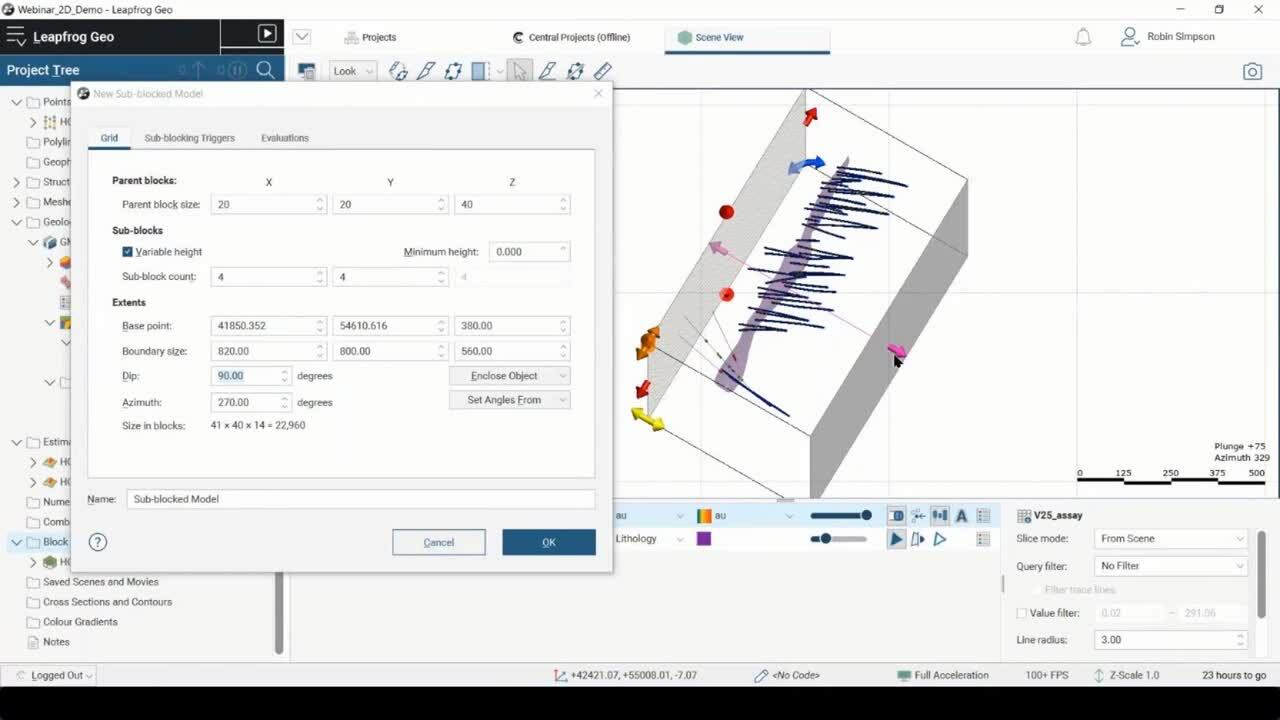
obviously you want to set up a block model.

[00:12:45.360]
In this case it may be useful to, rotate the block model

[00:12:51.070]
so that the Z dimension becomes matches the,

[00:12:55.260]
the thin dimension of the domain.

[00:12:57.760]
So, you have an example of that.

[00:13:06.207]
But the drill hole in 16 spacing here is on,

[00:13:11.140]
about 50 by 50.

[00:13:13.530]
So, there’s an example of, I’ll sit my block model

[00:13:15.660]
to be 20 by 20, I’ll have variable height, zits of locking,

[00:13:25.060]
and you get that zit, in the east west directions

[00:13:29.610]
of the vertical direction, into rotate the block model.

[00:13:41.000]
And then the extents become a bit difficult

[00:13:42.740]
to, give track of if you just follow the numbers so

[00:13:45.720]
best to do this,

[00:13:51.170]
in the, the scene view.

[00:14:00.170]
Okay.

[00:14:08.950]
We can go to, quite a small sub block size here, naked

[00:14:18.230]
by two blocks, sub-blocks and the north south

[00:14:21.800]
and vertical dimension.

[00:14:24.821]
And then the Kobo to one by one from model the small

[00:14:28.620]
without taking too much processing.

[00:14:34.200]
Yup, there’s numbers.

[00:14:42.280]
It’s possible just to have one block, one big block

[00:14:45.790]
in the, within dimension that then we let

[00:14:49.378]
the variable sub-blocking or it’s work

[00:14:52.180]
so we had just one block of the exact thickness

[00:14:54.640]
of the vein, which in this case,

[00:14:56.860]
the, but this main structure here

[00:14:58.200]
is about 1.2 meters thick on average.

[00:15:02.890]
Okay, so that,

[00:15:03.983]
that then I’ll set my, sub blocking triggers based

[00:15:08.010]
on the geological model and do an evaluation based

[00:15:11.300]
on that as well.

[00:15:18.760]
And that creates the, the sub-block model

[00:15:21.580]
that we’re now going to, throughout creating estimation.

[00:15:38.139]
And that looks reasonably good.

[00:15:45.430]
Are you sure you don’t have to use

[00:15:46.560]
that variable, height sub-blocking, for 2D estimation

[00:15:52.027]
and you can have a recurrence sub-block.

[00:15:55.130]
I just find the variable height sub-block

[00:15:58.750]
in this case, is often results

[00:16:02.610]
in smaller file sizes that still get a good fit

[00:16:05.984]
to the wireframe with reasonable processing times

[00:16:10.860]
but it’s not essential.

[00:16:12.800]
You can have regular sub-block as well.

[00:16:20.680]
So that’s set up the block model.

[00:16:22.590]
Now the actual 2D estimation workflow itself, as I said

[00:16:26.330]
the pre prerequisites are, you’ve got an essay table

[00:16:29.870]
and you’ve got a geological model.

[00:16:33.300]
First step, is to evaluate the geological model

[00:16:37.280]
under the database.

[00:16:40.940]
So that’s my model that has vein 25 in it.

[00:16:47.820]
And it just accept the defaults.

[00:16:54.090]
And after you’ve created this evaluation,

[00:16:57.280]
then you need to create a merge table

[00:16:59.750]
between the essay table and the evaluation.

[00:17:14.561]
Then once you have the merge table, set up a filter,

[00:17:19.650]
so you can select your domain code,

[00:17:42.900]
and then once you have got the filter, composites

[00:17:47.250]
and we use the economic compositing,

[00:17:51.070]
function to get a full length composite.

[00:17:56.620]
Now the input will be the grade

[00:18:00.210]
from that merge table we’ve created

[00:18:03.260]
and with the filter you’ve just created.

[00:18:07.000]
And then in the compositing additions, we’ll use a bit

[00:18:12.110]
of a trick here, which is we have effectively zero cutoff

[00:18:16.180]
grade,

[00:18:18.297]
and zero minimum length.

[00:18:22.860]
And that enables, everything that’s being captured

[00:18:27.270]
by the domain filter, to be in the composite.

[00:18:29.570]
We’re not actually putting any grade or thickness conditions

[00:18:31.970]
in here.

[00:18:35.300]
Or you can do some capping here.

[00:18:37.500]
In this case, I chose a cap of 90.

[00:18:41.730]
And remember that’s a capping on the raw,

[00:18:46.520]
the raw essays, not on any kind of composites.

[00:18:55.660]
So that sets up the economic composite,

[00:19:04.630]
which,

[00:19:07.790]
the table itself, has the following attributes,

[00:19:13.670]
from two gold,

[00:19:16.050]
through length.

[00:19:18.050]
Now, actually there’s one more thing I should add

[00:19:21.767]
about the economic composites.

[00:19:29.172]
You want to use true thickness,

[00:19:31.210]
and we use a plane that’s rotated.

[00:19:35.020]
So getting the true thickness and that thin dimension

[00:19:38.010]
of the vein, which in this case,

[00:19:42.570]
so in general, it’s dipping vertically striping north south.

[00:19:50.650]
Do that one again.

[00:20:02.900]
Okay, there we have it.

[00:20:04.190]
So we have,

[00:20:06.660]
a table of economic composites as from and to,

[00:20:12.220]
gold grade, a true length, which is calculated based

[00:20:17.240]
on that plane, we set up in the compositing,

[00:20:20.830]
the previous ones the orientation linear grade,

[00:20:24.040]
which is what I’ve been calling accumulation before,

[00:20:26.520]
but that’s the product of the gold and the true length.

[00:20:32.890]
The rest of the other fields, aren’t really relevant

[00:20:37.340]
in this case.

[00:20:43.480]
Now the next step, that will enable us to keep

[00:20:47.640]
the whole process dynamic, is we use

[00:20:50.520]
the new interval midpoints to, select from

[00:20:56.030]
that economic composites file.

[00:21:00.850]
So we can select all, but the key ones we’re going to

[00:21:04.240]
be interested in are actually really only true length

[00:21:06.880]
and when you grade.

[00:21:13.320]
So that gives us the points,

[00:21:22.056]
do a check now on here, how this is looking.

[00:21:25.470]
So this is, the main wireframe.

[00:21:30.790]
These midpoints are a 2D composites,

[00:21:35.830]
dragon linear grade.

[00:21:48.430]
So that’s showing us it’s all pretty good so far,

[00:21:55.590]
with the 2D composites aligning quite well

[00:21:59.030]
with where the drill holes, pierce the wireframe.

[00:22:09.320]
So now the estimation,

[00:22:13.640]
new domain estimation,

[00:22:16.620]
the domain will be that,

[00:22:19.260]
that the domain from our geological model, the input value,

[00:22:24.530]
is, comes from the mid points.

[00:22:30.140]
I noticed here when you’re selecting the input

[00:22:33.897]
you don’t usually get the, economic compass appearing here.

[00:22:36.810]
So that’s, that’s all we needed to add that midpoint step

[00:22:39.360]
to keep it all dynamic.

[00:22:41.680]
So linear grade, which is different word

[00:22:45.130]
for accumulation,

[00:22:56.433]
check on the statistics.

[00:23:03.040]
So 45 points that matches the number of drill holes

[00:23:07.313]
to seating, so that’s good.

[00:23:12.093]
When you’re grinding up grades,

[00:23:14.160]
so these are products and grades and thickness.

[00:23:22.190]
And we’ll need to, establish a variogram model.

[00:23:31.120]
Now, the orientation of the variogram model should match

[00:23:34.690]
the orientation we’ve, we use for that plane

[00:23:39.760]
and a 2D composites, so the, the vertical plane,

[00:23:44.900]
north south.

[00:24:02.970]
<v ->Sometimes it’s really creaking, It can be tricky</v>

[00:24:05.280]
to come up with a variogram model

[00:24:09.013]
because you’re only working with full moon sections

[00:24:11.630]
you don’t have that many points to work with.

[00:24:15.620]
And there’s be a bit of guessing involved,

[00:24:18.490]
how to set up the very grand model, and guessing

[00:24:21.870]
isn’t always the worst approach.

[00:24:23.493]
I mean, so, you can still make reasonable assumptions

[00:24:29.410]
about what a nugget proportion would be,

[00:24:32.450]
what the range would be based on your knowledge

[00:24:34.870]
of the deposits and the structure of this case.

[00:24:40.090]
A few hundred meters to the west of this plane,

[00:24:44.290]
there was another vein where there was part

[00:24:47.640]
of the same resource model, where we had quite a lot

[00:24:51.210]
of, or many years of channel sampling.

[00:24:53.740]
They gave us, a resolution of intersections

[00:24:57.770]
over just a few meters.

[00:24:58.960]
So, we were able to borrow the variogram model

[00:25:02.990]
from another domain for this domain.

[00:25:06.840]
Well, roughly set up a variogram model to use here.

[00:25:10.450]
So i give it 30% and I get,

[00:25:15.180]
a range of,

[00:25:18.920]
150,

[00:25:21.660]
100 and the major and semi major erections.

[00:25:27.780]
And to get the 2D effect to work.

[00:25:31.390]
The counterintuitive thing to do,

[00:25:33.840]
is actually to give a very large number

[00:25:37.580]
in the minor field.

[00:25:40.600]
So that is the effect of flattening everything out

[00:25:43.820]
in dimension.

[00:25:49.750]
Look at that now,

[00:25:58.967]
was a bit of a plunge to this structure, ’cause you know

[00:26:01.762]
about, moderately plunging to the north.

[00:26:06.330]
So I’ll put that in the variogram model as well.

[00:26:19.970]
This is a video looking west and you can see as does seem

[00:26:24.730]
some sort of tendency for the higher grades

[00:26:27.550]
to have that moderate plunge to the north.

[00:26:34.040]
So they’ll put my ellipsoid on, that’s how I’m capturing

[00:26:37.460]
it for the variogram model.

[00:26:47.410]
I think that various grams could enough now,

[00:26:52.660]
then we create a pre-estimator.

[00:27:02.310]
The options,

[00:27:04.980]
from a rotation of the block model at the start,

[00:27:08.040]
is our thin dimension,

[00:27:09.850]
and in the context of 2D estimation,

[00:27:14.200]
this realization of Z makes most sense just to have one

[00:27:18.190]
but then you probably want to bump up dis colorization

[00:27:21.157]
and the two other directions.

[00:27:25.600]
Tapping,

[00:27:28.060]
you can potentially add a cap here.

[00:27:30.440]
Remember, this is a cap on the accumulation

[00:27:32.830]
and not the grades.

[00:27:35.620]
I’ve already included a cap,

[00:27:38.090]
on the raw samples, when I set up the composite step,

[00:27:43.900]
so I’ll just leave, do nothing there.

[00:27:50.530]
Search neighborhood, I’ll start with my variogram model.

[00:27:56.860]
Doesn’t have to match the variogram model, proportional.

[00:28:03.000]
And again, it’s of a 2D effect to work,

[00:28:06.833]
the trick is to have a higher value

[00:28:09.970]
in that measurement field search.

[00:28:18.010]
Well, because we generally with fall into sections

[00:28:20.250]
and not say one minute composites, generally,

[00:28:25.360]
you can work with much lower maximum number of samples

[00:28:28.850]
than you would normally set aside, just six here.

[00:28:35.310]
We’ll put one there for now,

[00:28:40.404]
and on the output,

[00:28:43.040]
I’m maybe interested to see the number of samples.

[00:28:49.130]
I’m setting this up as a single pass, estimation.

[00:28:54.020]
You can certainly do multiple pass estimations

[00:28:56.400]
but to keep it simple or just to one pass here.

[00:29:10.840]
So once you’ve created that estimator, by some linear grade,

[00:29:17.330]
then,

[00:29:18.770]
copy the whole estimation and keep everything

[00:29:23.970]
the same except change the input variable

[00:29:27.650]
to the, true length of the thickness.

[00:29:42.700]
Now, in general, you should aim to have exactly

[00:29:45.760]
the same variogram model and the same search neighborhood

[00:29:51.500]
for both the accumulation and the thickness parts

[00:29:54.910]
of the estimate.

[00:30:00.157]
Don’t, they can be some strange results too,

[00:30:05.570]
when you get to the backyard version, grade part.

[00:30:08.540]
So,

[00:30:10.720]
don’t be too fancy with trying to get,

[00:30:14.190]
with a different variogram model for the thickness.

[00:30:23.360]
So we’ve got those, two tourist motors now,

[00:30:28.140]
I will go to the block model,

[00:30:31.580]
and evaluate.

[00:30:34.260]
using those estimators.

[00:30:45.262]
And that’s quite quick for this just one domain

[00:30:49.140]
and not too much sub-blocking.

[00:30:57.603]
I put the block model back on.

[00:31:02.686]
And I’ll just check that it fully informed.

[00:31:15.180]
Right, I don’t see any of the default purple color

[00:31:19.160]
for blocks that we had estimated.

[00:31:21.020]
So that search neighborhood was big enough

[00:31:22.730]
to get everything in one pass.

[00:31:28.690]
So almost there with calculation right now,

[00:31:30.930]
so in the box model the calculations

[00:31:32.710]
and filters, numeric calculation,

[00:31:45.050]
and the grade is, we divide our accumulation estimate

[00:31:48.670]
by our thickness estimate.

[00:31:58.570]
And there it is.

[00:32:07.220]
So a quick check looks reasonable compared

[00:32:09.840]
to the, input composites.

[00:32:13.350]
It looks reasonable compared to that assumption

[00:32:15.950]
of north plunge,

[00:32:20.390]
to the mineralization.

[00:32:25.150]
And these 2D estimates are actually, a bit easier

[00:32:28.750]
to validate visually than a 3D estimate for a narrow domain

[00:32:34.000]
because, we’ve got the same grade across the full thickness,

[00:32:40.380]
which has only, one meter or so on average for this mine.

[00:32:45.060]
Whereas if we did a 3D estimate,

[00:32:48.170]
it would be a bit more confusing

[00:32:49.520]
because we could have changing block boundaries

[00:32:52.650]
and changing grades across that, narrow dimension.

[00:33:02.318]
So that’s the process in Leapfrog,

[00:33:04.040]
I’ll go back to, PowerPoint and just summarize what I did.

[00:33:09.529]
So to start, the prerequisites, the assay table,

[00:33:11.683]
geological model.

[00:33:14.110]
Set up a block model, possibly you may want

[00:33:16.610]
to use some rotation to orientate the Z variable

[00:33:21.550]
sub-blocking height to be in the thin dimension.

[00:33:25.257]
And then put your geological model triggers and evaluation

[00:33:28.790]
of the block model, evaluate the geological model

[00:33:33.260]
onto the database.

[00:33:35.190]
This is the first, first step

[00:33:36.880]
of the 2D estimation workflow.

[00:33:40.740]
Create the merged table

[00:33:42.190]
of the evaluation and essays, set up a filter

[00:33:45.590]
on that merged table to match the domain,

[00:33:48.890]
use economic compositing, with that merged table

[00:33:54.220]
and the filter on zero cutoff and zero in on thickness.

[00:34:00.330]
Create points from the economic composites

[00:34:03.680]
and then set up the estimations for, maybe a grade

[00:34:07.750]
and copy that estimation to create the estimation

[00:34:11.140]
for thickness.

[00:34:13.200]
Evaluate those serious motions

[00:34:14.620]
onto the block model, and then divide

[00:34:18.750]
the accumulation estimate by the thickness estimate

[00:34:22.370]
to obtain your bad calculator grade.