


The objective of this example is to verify the simulated change in pressure of a constant volume of dry air subject to an increase in temperature. The temperature increase is simulated by TEMP/W while the air pressure response is simulated by AIR/W. The numerical simulation can be described as loosely coupled since the temperature change affects air pressure but the air pressure does not influence the temperature.
Background
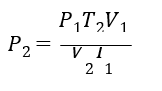
The combined gas law can be used to compare the state of a gas at two different conditions:
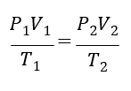
where 𝑃 is the absolute pressure of the gas, 𝑉 is the volume, and 𝑇 is the absolute temperature. The combined gas law is based on the ideal gas law, which is an equation of state:
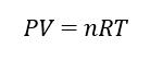
where 𝑛 is amount of gas in moles and 𝑅 is the universal gas constant (8.3144598(48) J mol−1 K−1). The ideal gas law can be rearranged to determine the density (𝜌) of the gas:
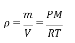
given the substitution 𝑛 = 𝑚/𝑀, where 𝑚 is the mass of gas and 𝑀 is the molecular mass of the gas. The molecular mass of dry air is assumed as 0.02897 kg mol−1.
Numerical Simulation
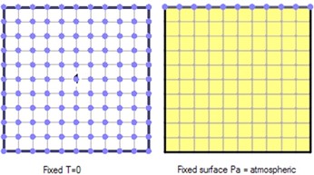
The associated project file comprises two coupled AIR/W and TEMP/W analyses; one that is steady- state and the other that is transient. The steady-state analysis establishes the initial temperatures and air pressures within the domain. An initial air temperature of 0°C is specified over the entire domain and an air pressure of 0 kPa is applied at the top boundary (Figure 1).
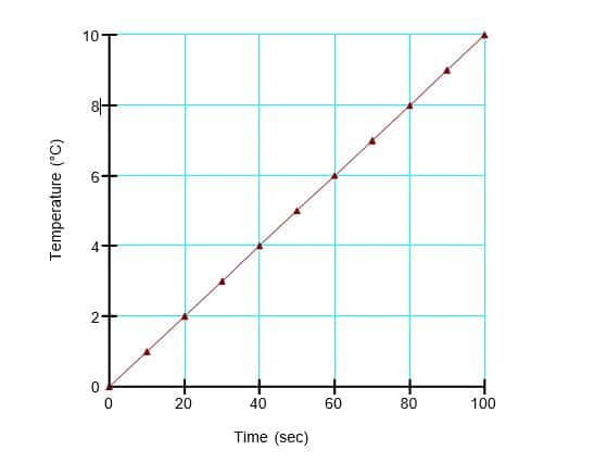
In the transient analysis, a cubic meter of dry air in a closed system is heated by 10°C for a duration of 100 seconds in 10 steps. A time-based function is used to increase the temperature from 0°C to 10°C over the modeled duration (Figure 2). The temperature boundary condition is applied to all nodes in the domain. All four boundaries of the domain have an unspecified air transfer boundary condition and therefore represent no-flow boundaries. Air cannot leave the domain during this transient analysis; consequently, the air pressure must increase as the domain warms.
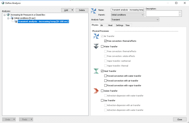
In this example, the air and heat transfer options are activated in both analyses. In the transient analysis, the ‘Free convection: thermal effects’ option is also activated (Figure 3). The air transfer
formulation will consider the affects of temperature on the air stored within the domain. Again, the system is closed, which means that air pressure must increase in order for the volume to remain constant.
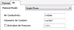
The material properties must be defined for the air and heat transfer processes. In AIR/W, a single phase or dual phase material model can be selected based on the complexity of the analysis. In this case, the single phase air material model is used to define the air conductivity and volumetric air content. The air conductivity is specified as 1 m s-1, and a volumetric air content of 1 m3 m-3 is inputted as the domain is only comprised of dry air (Figure 4). The value of air conductivity is inconsequential given that the system is closed and the air remains static.
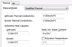
Temperature is specified at all nodes in the domain for both of the analyses so temperature is not dependent on the specified thermal material properties. Thus, a simplified thermal material model is
selected and a value of 1 was inputted for both the thermal conductivity and volumetric heat capacity (Figure 5).
Results and Discussion
The objective of this example is to confirm that the simulated results follow theoretical relationships for an ideal gas. The combined gas law can be used to calculate an exact solution for the final air pressure in the system:
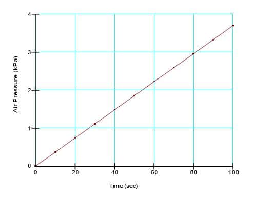
where 𝑇1 is 0°C, 𝑇2 is 10°C, 𝑃1 𝑉1 and 𝑉2 cancel). The calculated final air pressure is 3.7 kPa. The simulated air pressure at the top of the closed system at the end of the secondary analysis was 3.696 kPa (Figure 6).
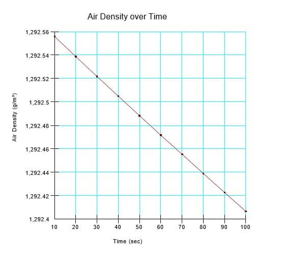
Both the mass and volume of air are constant during the transient simulation; consequently, the density should remain constant (Figure 7). The simulated density drifted very slightly from the 10
second value because of the nature of finite element formulations. Discretization in time results in a finite element formulation that contains a degree of solution accuracy that is dependent on time step size. The computed air density decreases negligibly by -0.15 g/m3, giving a final density that is in theoretical agreement with the simulated pressure of 3.696 kPa (i.e. slightly less than the theoretical value of 3.71 kPa). Increasing the number of time steps from 10 to 100 causes the change in density to decrease to -0.013 g/m3. Regardless, the change in density is negligible.
Summary and Conclusions
This example verifies the coupled AIR/W and TEMP/W formulation by simulating the response of a closed system containing air subject to a temperature change. The simulated air pressure change was marginally smaller that the theoretical value calculated via the combined gas law. This negligible discrepancy was reflected perfectly in the simulated air density and is the result of discretization in time.