Using Leapfrog Edge for dynamic grade control in underground mines

Join us for a 30-minute webinar on Using Edge for Underground Grade Control. The presentation will include an overview of the Edge block modelling extension, its place in the Seequent solution, and examples of workflows for short term planning and ore control.

Overview

Video Transcript

[00:00:00.166]
(upbeat music)

[00:00:03.552]
<v Steve>Thank you for taking the time today</v>

[00:00:05.550]
to listen to this webinar.

[00:00:07.750]
My name is Steve Law and I have been

[00:00:09.610]
a Senior Project Geologists with Seequent

[00:00:12.150]
for the past two and a half years.

[00:00:14.750]
I am the Technical Lead for Leapfrog Edge

[00:00:17.290]
and new product Pro 3D.

[00:00:20.300]
My background is primarily as a Senior Geologist

[00:00:23.120]
in Production and Resource Geology roles.

[00:00:27.480]
I will be presenting an example workflow

[00:00:30.040]
of how to use Seequent Mining Solutions software

[00:00:33.410]
to enhance the Grade Control process

[00:00:35.810]
in an underground operating environment.

[00:00:38.590]
Most aspects could also be utilized

[00:00:40.730]
in an open cut operation as well.

[00:00:44.330]
The key point of today’s demonstration

[00:00:46.640]
is to show the dynamic linkages

[00:00:48.340]
between Leapfrog Geo and Leapfrog Edge

[00:00:50.980]
managed within the framework of Seequent Central.

[00:00:54.770]
I will briefly touch on data preparation

[00:00:56.980]
and an example of workflow

[00:00:58.670]
splitting projects by discipline.

[00:01:01.540]
While it’s not designed as a training session,

[00:01:03.970]
I will cover the basic domain centric setup within Edge

[00:01:07.230]
and show the different components, including variography.

[00:01:12.350]
I will focus a little more on the Block Model setup

[00:01:14.900]
and how to validate the Grade Control Model

[00:01:17.580]
and report results as this part of the workflow

[00:01:20.430]
is a little different to how you may be used to doing it.

[00:01:25.200]
The Seequent Solution encompasses

[00:01:27.040]
a range of software products

[00:01:28.840]
applicable for use across the mining value chain.

[00:01:32.640]
Today I’ll focus on Seequent Central,

[00:01:34.880]
Leapfrog Geo and Leapfrog Edge,

[00:01:37.390]
which integrated together present the opportunity

[00:01:39.830]
to deliver key messages to different stakeholders.

[00:01:43.400]
Leapfrog Geo remains the main driver,

[00:01:46.010]
but I will show how by utilizing

[00:01:47.630]
the benefits of Edge and Central,

[00:01:50.130]
the workflow in an Underground Grade Control environment

[00:01:53.180]
can be enhanced.

[00:01:56.270]
Grade Control is the process

[00:01:57.810]
of maximizing value in reducing risk.

[00:02:00.820]
It requires the delivery of tons

[00:02:02.730]
in an optimum grade to the mill

[00:02:05.100]
via the accurate definition of ore and waste.

[00:02:08.170]
It essentially comprises data collection,

[00:02:10.850]
integration and interpretation, local resource estimation,

[00:02:15.730]
stope design, supervision of mining,

[00:02:17.630]
and stockpile management and reconciliation.

[00:02:22.550]
The demonstration today will take us up to the point

[00:02:25.320]
where the model would be passed

[00:02:26.570]
on to mine planning and scheduling.

[00:02:30.330]
The foundation of all Grade Control Programs

[00:02:32.830]
should be that of geological understanding.

[00:02:35.930]
Variations require close knowledge of the geology

[00:02:40.360]
to ensure optimum grade, minimal dilution

[00:02:43.210]
and maximum mining recovery.

[00:02:46.070]
By applying geological knowledge,

[00:02:48.180]
the mining process can be both efficient and cost-effective.

[00:02:53.280]
The integration and dynamic linkage of the geology

[00:02:55.940]
with the Grade Control Resource System

[00:02:58.170]
leads to time efficiencies.

[00:03:00.890]
We can reduce risk with better communication

[00:03:03.800]
via the Central Interface,

[00:03:05.840]
which offers a single source of truth

[00:03:07.670]
with full version control

[00:03:09.540]
member permissions and trackability.

[00:03:13.200]
Better decisions are achievable

[00:03:15.280]
as teams work together to collaborate

[00:03:17.380]
on the same data and models.

[00:03:19.710]
Everyone can discuss and explore

[00:03:21.320]
different geological interpretations

[00:03:23.320]
and share detailed history of the models.

[00:03:26.930]
Central provides a quality framework

[00:03:30.230]
for quality assurance as an auditable record

[00:03:33.450]
and timeline of all project revisions is maintained.

[00:03:37.590]
For those of you who have not been exposed

[00:03:39.560]
to Seequent Central, here is a brief outline.

[00:03:42.510]
It is a server based project management system

[00:03:45.340]
with three gateways for different users and management.

[00:03:49.240]
The Central portal is where administrators

[00:03:52.200]
can assign permissions for projects stored on the server.

[00:03:56.460]
Users will only see the projects

[00:03:58.100]
they have permission to view or edit.

[00:04:01.420]
The Central Browser allows users to view and compare

[00:04:04.790]
any version of the Leapfrog Project

[00:04:06.670]
within the store timeline.

[00:04:08.770]
The models cannot be edited,

[00:04:10.280]
but output meshes can be shared with users

[00:04:13.280]
who do not require direct access to Leapfrog Geo.

[00:04:16.920]
There is also a data room functionality,

[00:04:19.780]
which equates to a Dropbox type function

[00:04:22.080]
assigned to each project.

[00:04:24.990]
Today, I will focus on the Leapfrog Geo Connector,

[00:04:28.140]
which is where we can define various workflow structures.

[00:04:31.390]
Specifically, we will focus on one

[00:04:33.330]
where the projects are split

[00:04:35.360]
according to geology modeling or estimation functions.

[00:04:40.320]
I will now move on to the software demonstrations.

[00:04:44.870]
I have a project set up here,

[00:04:47.360]
which has been set up with three separate branches

[00:04:50.140]
a geology branch, an estimation branch,

[00:04:53.360]
and an engineering branch.

[00:04:55.250]
I will primarily be focusing

[00:04:56.620]
on the geology and estimation branches.

[00:05:01.020]
The way Central works is that you store

[00:05:02.630]
your individual projects on a server

[00:05:05.930]
and each iteration of the project

[00:05:08.380]
is saved in this timeline.

[00:05:10.500]
So the most recent project is always

[00:05:13.180]
the one at the top of the Branch.

[00:05:15.440]
So if we’re looking at Geology Branch here can see Geology,

[00:05:19.410]
we go to the top level of Geology.

[00:05:21.950]
And then this is the latest geology project.

[00:05:25.180]
Again, for estimation,

[00:05:26.930]
we followed through until we find the top most branch,

[00:05:30.750]
and this is the top most and most recent resource estimate.

[00:05:35.660]
To work with Central,

[00:05:36.830]
we download the projects by right clicking

[00:05:39.940]
on the required branch and they are then local copies.

[00:05:44.260]
So in this instance,

[00:05:45.440]
I have four local copies stored on my computer.

[00:05:48.650]
I am no longer connected to the cloud server

[00:05:51.470]
for working on these, I can go offline, et cetera.

[00:05:56.066]
The little numbers, 1, 2, 3, and four

[00:05:58.610]
refer to the instances up here.

[00:06:00.630]
So I always know which project

[00:06:02.640]
I’m working on at any one time.

[00:06:05.530]
For this demonstration,

[00:06:06.780]
I’m going to start off with the Geology model

[00:06:09.870]
as set up as a pre-mining resource.

[00:06:12.600]
So down here at Project 1.

[00:06:16.150]
So the data set we’re working with here

[00:06:18.670]
is a series of surface drill holes,

[00:06:20.720]
diamond drill holes, primarily.

[00:06:23.250]
And it’s basically a vein system.

[00:06:29.220]
And I have set up a simple series of four veins

[00:06:34.368]
as part of a vein system.

[00:06:38.770]
The main vein is Vein 1,

[00:06:40.790]
and then we have Veins two, three, and four

[00:06:43.320]
coming off as splice.

[00:06:47.660]
This model has been set up in a standard way.

[00:06:50.150]
So we have the geological model

[00:06:51.940]
and we’re going to use this

[00:06:53.770]
as the basis for doing an estimate

[00:06:56.020]
on veins 1, 2, 3, and four.

[00:07:01.210]
If you did not have Central,

[00:07:02.600]
then the Block Model would need to be created

[00:07:04.460]
within this project under the block models

[00:07:08.240]
and using the Estimation folder.

[00:07:10.430]
And then if you were going to update,

[00:07:13.310]
you would potentially freeze the Block Model

[00:07:16.690]
by using the new Freeze/Unfreeze function

[00:07:20.270]
and then to be updating the Geological model.

[00:07:23.050]
The Block Model won’t change until we unfreeze it.

[00:07:26.720]
The problem with this is that we don’t ever have

[00:07:32.030]
a record of what the previous model looked like

[00:07:34.180]
unless we zipped the project

[00:07:35.970]
and dated it and stored it somewhere.

[00:07:39.320]
The advantage of Central is that each iteration

[00:07:43.240]
is stored so that we can always go back

[00:07:45.460]
and see what the model looked like beforehand.

[00:07:49.090]
So the Geology Model has been set up.

[00:07:51.500]
I’m going to go now into the first estimation project

[00:07:58.500]
where I set up the pre-mining resource.

[00:08:00.520]
So in this case, this is local copy two,

[00:08:03.320]
and the branch is estimation.

[00:08:05.464]
(upbeat music)

[00:08:10.670]
The key difference here when using Central,

[00:08:12.890]
is that rather than directly linking

[00:08:15.160]
to a Geological Model within the project,

[00:08:17.870]
the domains are coming from centrally linked meshes.

[00:08:21.520]
So under the Meshes folder, you can see

[00:08:23.900]
we have these little blue mesh symbols.

[00:08:26.830]
And if I right click on these it’s reload latest on Branch

[00:08:31.960]
or from the project history.

[00:08:34.060]
The little clock is telling me that

[00:08:35.630]
since the last time I opened up this project,

[00:08:39.320]
something has changed in the underlying Geological Model.

[00:08:43.370]
Once we go reload, latest on project,

[00:08:46.180]
then the little clock will disappear.

[00:08:49.510]
So all the meshes that I’m using within the estimation

[00:08:53.530]
accessing directly from centrally linked meshes.

[00:08:58.540]
I’m just going to focus now on a quick run

[00:09:01.480]
through of how to set up a domain estimation

[00:09:04.530]
in Edge using Vein 1.

[00:09:09.980]
Edge works on a domain by domain basis.

[00:09:13.010]
So, and we work on one domain and one element,

[00:09:15.700]
and then we can copy and keep going through

[00:09:18.230]
until we create all four or more.

[00:09:22.310]
Each estimation is its own little folder.

[00:09:25.470]
So we have here, AU PPM Vein 1,

[00:09:30.530]
and we have within that a series of sub folders.

[00:09:34.120]
We can check quickly what the domain is

[00:09:36.670]
to make sure that we’re working in the space

[00:09:38.710]
that we expect to be.

[00:09:40.610]
And the values shows us the composites,

[00:09:46.630]
but it’s the midpoints of the intervals.

[00:09:48.670]
So it’s been reduced to point data,

[00:09:51.800]
which we can still display as normal drill holes.

[00:09:55.690]
And we can do statistics on that

[00:09:58.290]
and have a look at a histogram, et cetera,

[00:10:02.300]
Log Probability plots.

[00:10:06.470]
There is also a normal score functionality.

[00:10:09.700]
So if particularly when working with gold data sets

[00:10:12.870]
that are quite skewed,

[00:10:14.250]
we may wish to transform the values to normal scores.

[00:10:17.570]
So to do that,

[00:10:18.510]
we would right click on the values

[00:10:21.310]
and there will be a transformed values function

[00:10:24.970]
if it hasn’t been run already as it has been here.

[00:10:27.950]
So that produces a normal scores,

[00:10:30.960]
which is purely changing the data to a normal distribution.

[00:10:35.520]
And it decreases the influence of the high values,

[00:10:39.970]
whilst the variogram is being calculated

[00:10:42.996]
and is then back transformed into real space

[00:10:45.250]
before the estimate is run.

[00:10:51.570]
If we wish to edit our domain or our source data,

[00:10:55.380]
we can always go back to opening up at this level.

[00:10:58.420]
This is where we choose the domain.

[00:11:00.030]
And we can see here that it’s directly

[00:11:01.790]
linked back to the Central meshes here.

[00:11:06.260]
And then the numeric values

[00:11:08.160]
can come from any numeric table within our projects.

[00:11:11.520]
By the roar drill hole data or composite data if we have it,

[00:11:16.240]
but we have the option of compositing at this point,

[00:11:19.460]
which is what I’ve chosen to do.

[00:11:22.510]
The compositing done here is exactly the same

[00:11:25.220]
as if the compositing is done

[00:11:27.170]
within the drill hole database first,

[00:11:30.090]
it just depends on some processes

[00:11:31.920]
or whether it needs to be done there or here.

[00:11:34.835]
(upbeat music)

[00:11:38.290]
Variography done is all done

[00:11:39.400]
within the Special Models folder.

[00:11:41.730]
In this instance,

[00:11:42.563]
I’ve done a transformed variogram on the transform values

[00:11:46.020]
because it gives a better result.

[00:11:51.550]
The way we treat variography is too dissimilar

[00:11:53.910]
to other software packages.

[00:11:55.800]
We’re still modeling into three prime directions

[00:12:00.190]
relative to our plan of continuity.

[00:12:04.360]
The radial plot is within the our plane.

[00:12:08.880]
So in this case,

[00:12:09.840]
it’s set along the direction of the vein

[00:12:12.210]
and then we’re changing the red arrow.

[00:12:15.090]
It’s changing pitching plans.

[00:12:18.090]
The key thing when using Leapfrog is that the variogram

[00:12:21.580]
is always linked through to the 3D scene.

[00:12:26.370]
So if we move anything within forms,

[00:12:31.430]
then the ellipse itself will be changing

[00:12:34.050]
in the 3D scene and vice versa.

[00:12:36.420]
We can move the ellipse and it will change

[00:12:39.310]
the graphs in this side as well.

[00:12:43.760]
We have capability.

[00:12:46.020]
This is a normal scores one.

[00:12:48.180]
So once the modeling has been done

[00:12:50.530]
and we can manually change using the little leavers

[00:12:54.820]
or by just typing in the results through here

[00:12:57.940]
and hit save, we do need to use the back transform,

[00:13:01.480]
so that will process it.

[00:13:05.610]
So that is ready to use directly in the estimates.

[00:13:11.410]
Discard those changes.

[00:13:14.070]
Okay, another good feature that we have within Edge

[00:13:17.890]
is the possibility of using variable orientation,

[00:13:21.110]
which is effectively dynamic and atrophy.

[00:13:26.395]
So locally takes into account local changes

[00:13:30.080]
in the underlying domain geometry.

[00:13:34.860]
We can use any open mesh to set this up.

[00:13:40.280]
In this case,

[00:13:41.113]
I’m using a vein hanging wall surface to develop this.

[00:13:47.700]
This has been,

[00:13:50.170]
again, these surfaces have been imported

[00:13:52.840]
directly from the Geology Model

[00:13:55.760]
into a centrally linked meshes.

[00:13:57.970]
So as the geology model changes,

[00:13:59.800]
these will also be able to be updated if necessary.

[00:14:05.010]
There was a visualization of the variable orientation,

[00:14:11.730]
and that is in the form of these small disks,

[00:14:15.800]
which you can define on a grid

[00:14:18.370]
and you can display dip direction or dip.

[00:14:23.020]
And if we have a look in a section,

[00:14:28.960]
we can get an idea of how the ellipsoid will change.

[00:14:33.250]
So in this way,

[00:14:34.083]
the variogram will move through

[00:14:36.930]
and change its orientation relative to the local geometry,

[00:14:40.410]
rather than having to be set

[00:14:41.910]
at that sort of more averaged orientation

[00:14:45.430]
across the whole vein.

[00:14:50.290]
Sample Geometry is a couple of declustering to

[00:14:54.000]
which I will not go into at this stage.

[00:14:56.810]
The key folder that we need to work with

[00:14:59.230]
is the Estimates folder.

[00:15:01.210]
And this is where we can set up either inverse distance,

[00:15:04.460]
Nearest Neighbor, ordinary or simple kriging,

[00:15:08.720]
or RVF estimated the same type of algorithm

[00:15:12.480]
that we use under our geological modeling

[00:15:14.600]
and numeric models.

[00:15:17.000]
In this instance, I’ve set up two passes for the kriging.

[00:15:20.950]
So I can open up both of those at the same time.

[00:15:24.339]
(upbeat music)

[00:15:28.700]
We can set top cutting at this level.

[00:15:31.170]
So in this case, I’ve cut top cut to 50.

[00:15:36.030]
We don’t have to do it there,

[00:15:37.580]
If we can’t, we could do it in the composite file earlier,

[00:15:40.880]
but it wouldn’t need to be done outside of Leapfrog first.

[00:15:44.290]
The interplant tells whether it’s ordinary kriging

[00:15:47.660]
or simple kriging, and we defined a discretization,

[00:15:51.270]
which is based on the parent block.

[00:15:53.550]
So this is dividing the parent block that dimension

[00:15:56.360]
into four by four by four.

[00:15:59.680]
We picked a Variogram Model.

[00:16:01.480]
So it was only one to choose from.

[00:16:03.740]
The estimates can only see the variograms

[00:16:07.280]
that are sitting within the particular folder

[00:16:10.810]
that you’re working from,

[00:16:12.480]
but you can have as many different variogram models

[00:16:14.620]
as you like to choose from

[00:16:16.180]
and test different parameters.

[00:16:20.080]
The Ellipsoid, so when we first developed this,

[00:16:23.590]
it is usually set to the variogram,

[00:16:27.070]
and then in this case,

[00:16:28.730]
we are overriding it by using the variable orientation.

[00:16:32.350]
So it keeps maintains the ranges,

[00:16:35.180]
but changes the orientation as relative to the mesh.

[00:16:41.270]
You can see here that the second search that I’ve set up

[00:16:44.230]
is simply double the ranges of the first.

[00:16:48.960]
We have a series of fairly standard

[00:16:52.780]
search criteria and restrictions.

[00:16:55.200]
So minimum maximum number of samples,

[00:16:57.640]
outlier restriction, which is a form of top cutting,

[00:17:01.940]
but not quite as severe.

[00:17:03.500]
So you only top cutting

[00:17:06.280]
high values beyond a certain distance.

[00:17:09.220]
Sector search as both Oakton or quadrant

[00:17:12.410]
and Drillhole limit,

[00:17:13.650]
which is maximum number of samples per drill hole.

[00:17:17.100]
In this case of telling this effectively

[00:17:20.160]
says that I must have at least one drill hole to proceed.

[00:17:28.240]
The second search is looking at a greater distance,

[00:17:31.190]
reducing down to number one sample and no restrictions.

[00:17:34.550]
And this is simply to try and get a value

[00:17:37.020]
inside all the blocks, which is needed

[00:17:39.210]
for reporting later on.

[00:17:41.930]
One point of difference for Edge compared to other software

[00:17:45.010]
is how we define variables.

[00:17:47.390]
So the grade variable name is this name down here,

[00:17:51.020]
which is automatically assigned,

[00:17:52.680]
but can be changed then rather than having

[00:17:55.930]
to set up variables within a Block Model definition,

[00:17:59.200]
we simply tick the boxes for the ones

[00:18:01.240]
that we may want to store.

[00:18:02.800]
So if we want to store kriging variance,

[00:18:04.670]
we’d simply tick the box here.

[00:18:07.190]
It doesn’t matter if we don’t tick it individually

[00:18:09.580]
and decide you need it later.

[00:18:10.850]
You can always come back to here

[00:18:12.450]
and tick the boxes as necessary.

[00:18:15.010]
I find that it is useful not to tick them

[00:18:17.750]
if you don’t need them,

[00:18:19.370]
’cause it makes the processes quite busy later on.

[00:18:23.920]
So let us set up the parameters.

[00:18:26.470]
So estimation folder can be thought of as a parameter file.

[00:18:32.610]
And this is where we set up

[00:18:33.540]
all the parameters for our estimate.

[00:18:36.640]
One key concept that we need to understand

[00:18:40.350]
is the concept of a combined estimator.

[00:18:44.350]
If I evaluate or view these runs,

[00:18:47.790]
Run 1 and Run 2 in the Block Model,

[00:18:50.140]
I’ll only be able to display either one,

[00:18:52.360]
Run 1, or Run 2 at a time,

[00:18:55.300]
as well as I’ve got four veins set up.

[00:18:58.490]
I can only see each vein individually.

[00:19:01.220]
So I need to combine them together

[00:19:03.860]
to be able to view the whole goal grade

[00:19:06.560]
of everything at once.

[00:19:08.210]
And this is done by creating a new combined estimator,

[00:19:11.450]
which is simply like a merged table

[00:19:13.640]
from the geological database.

[00:19:16.130]
So in this instance, I’ve set up all of the veins,

[00:19:20.390]
and each pass for each.

[00:19:22.600]
The order of the domains isn’t critical

[00:19:25.300]
because they’re all independent of each other,

[00:19:27.950]
but the order of the passes is very important.

[00:19:31.220]
So Pass 1 must be on top higher priority,

[00:19:35.320]
and then that means that that is looked at first

[00:19:38.910]
then any blocks that do not have a value in them

[00:19:41.280]
after that is run, we’ll then use the Pass 2 parameters.

[00:19:45.470]
If we inadvertently price Pass 2 above,

[00:19:48.720]
then it festively overrides Pass 1.

[00:19:52.680]
It is re-estimating every block with Pass 2 parameters

[00:19:56.810]
as it does it.

[00:19:57.870]
So the order is quite important.

[00:20:03.610]
As you add new domains,

[00:20:06.170]
then you can simply select that’ll be available

[00:20:09.210]
over here on the left, and you can move them across at will.

[00:20:17.360]
Okay, this is often the variable that is exported

[00:20:20.720]
to other software packages in a Block Model.

[00:20:23.090]
So I tend to try and keep

[00:20:24.270]
the naming of these quite short and simple,

[00:20:26.920]
because a lot of packages are limited

[00:20:28.490]
to how many characters they can accept.

[00:20:31.210]
Again, outputs can be calculated

[00:20:33.240]
for the combined estimate

[00:20:35.640]
so we can store any of these.

[00:20:37.440]
And it does automatically assign an estimator number

[00:20:41.520]
and a domain number.

[00:20:44.490]
So if we have two passes,

[00:20:46.780]
then will slightly code the passes

[00:20:49.460]
slightly different shades.

[00:20:51.710]
In this instance,

[00:20:52.543]
like pass one and two slightly different grades of Aqua.

[00:20:58.620]
Since we have all our estimates

[00:21:00.090]
and combined estimator set up,

[00:21:02.120]
we then proceed to setting up a Block Model.

[00:21:06.200]
And this is where we view, validate, and report.

[00:21:09.860]
The validation Swath plots, and the resource reports

[00:21:15.420]
are all embedded within the Block Model.

[00:21:18.110]
And so when the Block Model updates,

[00:21:20.860]
these ancillary functions update as well.

[00:21:28.660]
In this case, we’re using a Sub-Block Model.

[00:21:30.990]
We can do regular models, which is simply a new block model.

[00:21:35.100]
It’s exactly the same, except in for a sub-block model,

[00:21:38.170]
we have sub block count,

[00:21:39.930]
which is the parent block size divided by the count,

[00:21:42.560]
so in this case, we’ve got 10 meters, parent blocks,

[00:21:45.930]
and two meter sub-blocks in all directions.

[00:21:50.830]
Sub-block models can be rotated in both deep and estimate.

[00:21:54.640]
Sub-blocking triggers is important.

[00:21:57.320]
So for us, we are bringing across the meshes of each vein.

[00:22:02.100]
So if we add a new vein,

[00:22:03.920]
we would need to bring that across to the right-hand side.

[00:22:07.780]
And then the most important tab is the Evaluations tab.

[00:22:12.110]
Anything that we want to see in the Block Model or run

[00:22:15.683]
needs to come across to the right-hand side.

[00:22:18.700]
So in this case, we are running the kriging

[00:22:23.610]
for Pass 1 in each of the veins,

[00:22:26.800]
and I’ve got the combined estimator.

[00:22:28.980]
Now I do not need to bring across the individual components

[00:22:32.910]
if I have a combined estimator,

[00:22:34.970]
it’s just that I want to look at the underlying composites

[00:22:39.530]
against the estimate in a Swath plot,

[00:22:41.730]
I can only do so with the underlying individual run files,

[00:22:47.370]
not the combined estimator,

[00:22:49.890]
but so for validation, I do need the individuals.

[00:22:53.950]
And normally I would just look at Pass 1,

[00:22:57.160]
but if I’m just reporting,

[00:22:58.460]
I don’t not need these and I can remove them

[00:23:01.470]
and take them across to the left

[00:23:03.020]
and would just have the combined estimators.

[00:23:06.770]
So whenever a new parameter is set up

[00:23:09.290]
in the Estimation folder,

[00:23:10.970]
then you must go to the corresponding block model

[00:23:13.800]
and move it across to the right

[00:23:16.260]
on the evaluation tab for it to run.

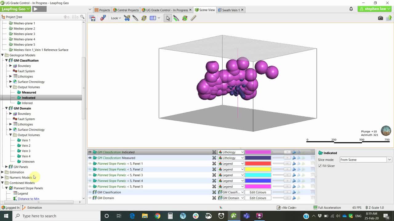
[00:23:21.940]
To visualize our results,

[00:23:27.590]
we have got all of the evaluations

[00:23:30.480]
that we’re told it to use.

[00:23:32.130]
This is our combined estimator, so we can see,

[00:23:41.840]
I can see the results of all four veins,

[00:23:45.760]
and there are some other tools here against H parameter.

[00:23:52.570]
We’ve got this status.

[00:23:54.080]
So if we have a look at Vein 1 by itself,

[00:23:57.350]
that’s that just shows the results for Vein 1,

[00:24:01.240]
and we can look at a status and this shows us

[00:24:07.730]
which blocks were estimated and which are not.

[00:24:10.040]
So we still have a few blocks around the edges

[00:24:12.950]
or from data that aren’t estimating at this stage.

[00:24:17.960]
Anything that we stored in the outputs,

[00:24:20.500]
so that number of samples can be displayed.

[00:24:24.070]
So we can see here that we’ve got

[00:24:25.540]
plenty of samples in the middle,

[00:24:27.260]
but it gets quite sparse around the edges.

[00:24:32.680]
Another feature of block models is calculations and filters.

[00:24:37.270]
So what this one is doing is

[00:24:39.570]
we store all the possible variables

[00:24:42.760]
that we may use within the calculation.

[00:24:45.390]
And in this one, I’ve made a new numeric calculation,

[00:24:49.590]
which says if there is a grade in the block,

[00:24:53.640]
then use that grade,

[00:24:55.030]
but if there is not make it 0.01.

[00:24:58.350]
So this is just one way of trying

[00:25:00.210]
to remove blocks that have not been estimated.

[00:25:04.430]
The other way would be to

[00:25:06.000]
could set up a Nearest Neighbor

[00:25:08.490]
with a large search and append

[00:25:10.920]
that to the combined estimator at the very end.

[00:25:14.810]
So multiple ways of dealing with sparse blocks.

[00:25:20.240]
In this case our calculation

[00:25:22.260]
can be viewed in the Block Model.

[00:25:24.760]
Variables are parameters that can be used in a calculation,

[00:25:28.420]
such as something like gold price,

[00:25:30.520]
but you can’t visualize it in the model.

[00:25:33.630]
And then filters are simply query filters

[00:25:38.070]
to find as we would in drill holes,

[00:25:40.010]
but it’s applying to the actual block model.

[00:25:43.660]
So I’ve created this gold final calculation,

[00:25:49.440]
and it can be displayed because it shows up down in here.

[00:26:00.720]
And we can see all that grades above two grams.

[00:26:06.629]
Okay, so that’s the basic setup

[00:26:08.208]
of the very first Resource Model.

[00:26:12.240]
So coming back to here, we would then be ready to,

[00:26:15.328]
we have some new Grade Control drilling.

[00:26:18.110]
So we go to the Geological Model

[00:26:20.790]
where that drilling was upended, choose number three.

[00:26:26.720]
So we have a series of Drillhole, Grade Control,

[00:26:30.260]
infill holes that have been drilled as a fan

[00:26:36.250]
from underground.

[00:26:40.470]
Whoever’s in charge of working

[00:26:42.265]
on the interpretation.

[00:26:47.090]
We’ve gone through each of the drill holes, new drill holes,

[00:26:50.160]
and using the tool selection that had already been set up,

[00:26:54.360]
could reassign according to which veins

[00:26:56.690]
things are related to.

[00:26:58.260]
And then the model will update.

[00:27:04.040]
One handy thing to do is we have linking meshes directly,

[00:27:08.810]
but we can’t link drill hole information at the moment.

[00:27:11.900]
So what I would often do at this stage

[00:27:13.670]
is export all of the information

[00:27:16.700]
from the drill hole data set.

[00:27:18.930]
I could then load it to the data room

[00:27:23.220]
associated with this particular project.

[00:27:26.517]
(upbeat music)

[00:27:34.310]
So each project in the portal has files folder.

[00:27:39.760]
And within this folder, which it works similar to a Dropbox,

[00:27:43.990]
you could put the current drill hole database files,

[00:27:48.070]
and then we could download those.

[00:27:50.740]
And that will be ready to import into our estimation folder.

[00:27:54.550]
This portal is also where we can assign

[00:27:57.440]
users to the project, and each project

[00:28:04.490]
can have its own specific users.

[00:28:07.350]
So we go back to

[00:28:11.750]
this one and have a look at the users.

[00:28:18.330]
We can see that we’ve got 1, 2, 3, 5 users,

[00:28:21.740]
and they are all editors.

[00:28:23.960]
You can have people who are only going to be able to view

[00:28:28.807]
a few of the project and they would use central browser

[00:28:31.040]
to do that, but they cannot edit anything, okay.

[00:28:36.830]
So going back to, we have updated the geology.

[00:28:41.330]
So we go back to our estimation and we would open that up

[00:28:48.640]
and reload the new drilling.

[00:28:52.390]
So we have two options.

[00:28:53.560]
If it’s brand new drilling that doesn’t exist

[00:28:55.720]
anywhere in the project,

[00:28:57.240]
then we could use the append function.

[00:29:00.490]
So appending the drill holes, if you’re accessing

[00:29:05.805]
a main database and everything’s added to that,

[00:29:09.550]
then you could reload.

[00:29:10.740]
And that will put in all the new holes

[00:29:12.700]
and any changes, okay.

[00:29:21.090]
So the drill holes are updated.

[00:29:23.830]
And then within the meshes folder,

[00:29:28.756]
all the veins that might’ve changed need to be updated.

[00:29:31.240]
So we just simply go reload latest on Branch.

[00:29:34.240]
And then the Block Model will then rerun

[00:29:37.750]
and we are ready to report and validate.

[00:29:43.430]
Swath plots are maintained within the Block Model itself.

[00:29:48.310]
So to start with, we can create a new Swath plot.

[00:29:53.340]
Once it’s been created,

[00:29:54.520]
it is stored down on the graphs and tables,

[00:29:57.870]
and then we can open it up at any time

[00:30:00.870]
and have a look at them.

[00:30:02.600]
It automatically creates the X, Y and Z directions.

[00:30:07.480]
And we can add as many or few items as we like

[00:30:11.240]
using the selected numeric items.

[00:30:13.720]
In this case,

[00:30:14.553]
I’m wanting to compare the kriging in Pass 1.

[00:30:17.720]
And I want to look at the original composites.

[00:30:20.300]
So to do that, I need to turn them on down here.

[00:30:25.500]
So you can see that I’ve got

[00:30:27.290]
the clips composite values showing in the red.

[00:30:31.980]
If I had an inverse distance estimator, I could add that

[00:30:36.940]
and then I could compare the kriging

[00:30:38.210]
against this inverse distance.

[00:30:43.610]
Okay, we’re ready to report against our Block Model.

[00:30:49.070]
The key to reporting within Leapfrog Edge

[00:30:52.270]
is that we need to have a Geological Model

[00:30:57.440]
with output volumes that can be evaluated.

[00:31:00.140]
So at this stage,

[00:31:00.973]
we cannot directly evaluate meshes.

[00:31:03.990]
So they need to be built into a Geological Model.

[00:31:07.870]
So in this instance, I have a GM domain,

[00:31:11.360]
which is simply taking the meshes directly,

[00:31:14.570]
as we can see using the new intrusion from surface,

[00:31:21.760]
and that builds them up.

[00:31:23.890]
It’s also a good way of being able to combine domains.

[00:31:27.530]
So if for instance, we wanted to estimate

[00:31:30.480]
Vein 2, 3, and 4 as a single domain,

[00:31:35.190]
then we could basically assign

[00:31:39.830]
whatever name is in the first lithology.

[00:31:42.490]
So I could call this kriging Zone 2,

[00:31:45.140]
and I can still leave this as Vein 2 here,

[00:31:48.090]
but I just use kriging Zone 2

[00:31:50.190]
as the first theology for all three,

[00:31:52.920]
and then my output volumes,

[00:31:54.320]
I would just have kriging Zone 2 and Vein 1,

[00:31:57.510]
I could have a single vein for that one.

[00:32:00.610]
So it’s a great way of being able to combine

[00:32:03.780]
our domains together to run estimates.

[00:32:08.110]
We often use classification and often we’ll have shapes

[00:32:11.850]
maybe generated in another software,

[00:32:14.020]
or we could use polylines within Leapfrog to create a shape.

[00:32:18.350]
In this instance,

[00:32:19.183]
I’ve just done a quick distance buffer

[00:32:22.320]
around the drill holes, and I have referenced that.

[00:32:25.460]
So then I end up with two output volumes

[00:32:30.390]
for a measured and an indicated area.

[00:32:34.880]
And the rest would be inferred.

[00:32:39.880]
The same for any stoping panels.

[00:32:42.580]
If we wish to report within shapes or drive shapes,

[00:32:46.960]
they need to be built into a Geological Model first.

[00:32:49.780]
So in this instance, I’ve generated some panels.

[00:32:55.830]
So we’ve got

[00:32:56.663]
panel 1, 2, 3, 4, 5, okay.

[00:33:04.149]
I needed this to be combined against mineralization shape.

[00:33:09.020]
So I’ve actually used the combined model

[00:33:14.160]
and I have the combined.

[00:33:18.460]
So I have the Stipe panels confined to Vein 1,

[00:33:22.910]
which I will report against.

[00:33:28.220]
So resource reports again

[00:33:30.030]
built within the Block Model itself.

[00:33:32.050]
So new resource report,

[00:33:33.970]
you can have as many as you wish stored.

[00:33:36.390]
And then once they’re there, you can open them up.

[00:33:39.457]
(upbeat music)

[00:33:48.650]
And in this case, I’ve got the domain Vein 1 Pass 1,

[00:33:52.180]
domain Pass 2 and measured indicated inferred.

[00:33:56.710]
And we’ve got Pass 2 is only inferred.

[00:33:59.510]
And for each of the panels.

[00:34:01.180]
These can be moved around

[00:34:02.320]
so if we wanted the classification

[00:34:04.000]
to be first measured indicated,

[00:34:07.400]
and then there’s two components to the inferred.

[00:34:10.420]
We can apply a cutoff as we have done up here,

[00:34:13.170]
and SG can apply it either as a constant value,

[00:34:16.570]
or if you’ve got a different SG per domain,

[00:34:19.430]
and you can set up a calculation to do that,

[00:34:22.010]
or if you’ve estimated SG,

[00:34:24.170]
it would be available within the dropdown here.

[00:34:29.110]
You can choose which columns you wish to look at.

[00:34:32.300]
So if you don’t want to see the inferred,

[00:34:34.170]
you could untick that one there.

[00:34:37.300]
Then the second report that we’ve generated

[00:34:39.950]
is one where we’re looking

[00:34:41.040]
at the results for all four veins.

[00:34:44.520]
So we’ve got Vein 1, 2, 3, and four,

[00:34:46.860]
and just per panels without any classification.

[00:34:50.370]
So you can mix and match the resource reports

[00:34:53.820]
to whichever you want to look at.

[00:34:58.090]
So the process would just continue

[00:35:00.040]
as the next stage of geology

[00:35:04.200]
could add in some more mapping or drilling update,

[00:35:08.540]
the Geology Model would then open up the estimation again,

[00:35:15.200]
make the changes, and then you will publish this back.

[00:35:20.900]
So once the change is made, you publish that here.

[00:35:26.000]
These are the objects that can be viewed in Central Browser,

[00:35:28.740]
but regardless of what you tick here, everything is stored.

[00:35:33.180]
You can then assign it to a value like Peer Review.

[00:35:38.500]
It’s going to store the entire project.

[00:35:41.430]
And then you choose which branch,

[00:35:44.010]
because I’m working on an earlier model,

[00:35:46.180]
I have to make a new branch,

[00:35:48.260]
but if I had been working from the last one,

[00:35:51.350]
it would automatically keep assigning it

[00:35:53.410]
to the Estimation Branch.

[00:35:55.280]
It’s always useful to put some comments in there

[00:35:57.460]
for what he wants to do.

[00:35:58.960]
And then usually only takes

[00:36:00.340]
a couple of minutes to upload to the server.

[00:36:06.290]
Thank you for your attention today.

[00:36:08.811]
(upbeat music)